Stitching together MODIS data
MODIS has been around for some 12 years. There are many products that have large time series over the whole globe which one can use to study things. So I might want to produce a a timeseries of the 8-day Gross Primary Productivity (GPP) product over say the UK. Moreover, I might want to change the projection to something more appropriate to the UK. The first thing to note is that the UK (OK, and Ireland, and I'm ignoring Gibraltar, the Falklands and the like!;-D) is spread over two tiles, h17v03 and h18v03. The MODIS product needs to be downloaded for both tiles, and then mosaicked/stitched together. So, this is what we want to do:
- Download the complete time series for the relevant tiles
- Stitch together the tiles
- Reproject to some useful projection
The output data ought to be in an easy-to-use format, for example a multiband GeoTIFF file, where each band represents a different period.
It is important to note that I shall be using the GDAL VRT format a lot, and this requires in this case, opening many HDF files simultaneously. For this to work, you need to have the installed HDF libraries correctly configured. See the section Driver Building on the GDAL website.
Getting the data
Although one can use the Reverb website to select and download data, it is also easy enough to just get what you need from NASA's FTP servers. You can have sophisticated download tools such as modisficator, but sometimes it's just easier to have a shell script that uses wget to get the data. Said script is grab_modis.sh, and uses Bash and wget. Going by our example, let's say we want to download two tiles, for a few years. We'd just use a Bash command for this. We note that the GPP product for TERRA has the code MOD17A2.005
for tile in h17v03 h18v03;
do
    for year in {2000..2011};
    do
        ./grab_modis.sh MOD17A2.005 $tile $year
    done
done
The previous commands will take a while to download the data. We can see that we have downloaded a bunch of files like
MOD17A2.A2005001.h17v03.005.2007356110650.hdf
MOD17A2.A2005001.h18v03.005.2007356112231.hdf
We can see what's in each file using gdalinfo
gdalinfo MOD17A2.A2005001.h17v03.005.2007356110650.hdf
Driver: HDF4/Hierarchical Data Format Release 4
Files: MOD17A2.A2005001.h17v03.005.2007356110650.hdf
Size is 512, 512
Coordinate System is `'
Metadata:
  HDFEOSVersion=HDFEOS_V2.9
  LOCALGRANULEID=MOD17A2.A2005001.h17v03.005.2007356110650.hdf
  PRODUCTIONDATETIME=2007-12-22T11:06:50.000Z
  DAYNIGHTFLAG=Day
  REPROCESSINGACTUAL=reprocessed
  LOCALVERSIONID=5.2.6
  REPROCESSINGPLANNED=further update is anticipated
  SCIENCEQUALITYFLAG=Not Investigated
  AUTOMATICQUALITYFLAGEXPLANATION=Passed was set as a default value. May or may not require further study
  AUTOMATICQUALITYFLAG=Passed
  SCIENCEQUALITYFLAGEXPLANATION=See http://landweb.nascom.nasa.gov/cgi-bin/QA_WWW/qaFlagPage.cgi?sat=terra for the product Science Quality status.
  QAPERCENTMISSINGDATA=0
  QAPERCENTOUTOFBOUNDSDATA=77
  QAPERCENTCLOUDCOVER=82
  QAPERCENTINTERPOLATEDDATA=0
  PARAMETERNAME=MOD_PR17A2
  VERSIONID=5
  SHORTNAME=MOD17A2
  INPUTPOINTER=MOD15A2.A2005001.h17v03.005.2007352013935.hdf, MOD17A1.1.A2005.h17v03.hdf, MOD12Q1.A2001001.h17v03.004.2004358134257.hdf, MOD17_ANC_RI11.hdf
  GRINGPOINTLONGITUDE=-15.4860189105775, -19.9999999949462, 0.0325645816154951, 0.0125638874822562
  GRINGPOINTLATITUDE=49.7394264948349, 59.9999999946118, 60.0089388384779, 49.7424953501575
  GRINGPOINTSEQUENCENO=1, 2, 3, 4
  EXCLUSIONGRINGFLAG=N
  RANGEENDINGDATE=2005-01-08
  RANGEENDINGTIME=23:59:59
  RANGEBEGINNINGDATE=2005-01-01
  RANGEBEGINNINGTIME=00:00:00
  PGEVERSION=5.2.8
  ASSOCIATEDSENSORSHORTNAME=MODIS
  ASSOCIATEDPLATFORMSHORTNAME=Terra
  ASSOCIATEDINSTRUMENTSHORTNAME=MODIS
  QAPERCENTGOODQUALITY=0
  QAPERCENTOTHERQUALITY=23
  HORIZONTALTILENUMBER=17
  VERTICALTILENUMBER=03
  TileID=51017003
  NDAYS_COMPOSITED=8
  QAPERCENTGOODPSN=0
  QAPERCENTGOODNPP=0
  NORTHBOUNDINGCOORDINATE=59.9999999946118
  SOUTHBOUNDINGCOORDINATE=49.9999999955098
  EASTBOUNDINGCOORDINATE=0.0166666666624637
  WESTBOUNDINGCOORDINATE=-19.9999999949462
  ALGORITHMPACKAGEACCEPTANCEDATE=2005-02-11
  ALGORITHMPACKAGEMATURITYCODE=Normal
  ALGORITHMPACKAGENAME=MOD17A2
  ALGORITHMPACKAGEVERSION=5
  INSTRUMENTNAME=Moderate Resolution Imaging Spectroradiometer
  PLATFORMSHORTNAME=Terra
  PROCESSINGDATETIME=2007-12-22T11:06:50.000Z
  LOCALINPUTGRANULEID=MOD15A2.A2005001.h17v03.005.2007352013935.hdf, MOD17A1.1.A2005.h17v03.hdf, MOD12Q1.A2001001.h17v03.004.2004358134257.hdf, MOD17_ANC_RI11.hdf
  GEOANYABNORMAL=False
  GEOESTMAXRMSERROR=50.0
  LONGNAME=MODIS/Terra Gross Primary Productivity 8-Day L4 Global 1km SIN Grid
  PROCESSINGCENTER=MODAPS
  NUMBEROFGRANULES=1
  GRANULEDAYNIGHTFLAG=Day
  CHARACTERISTICBINANGULARSIZE=30.0
  CHARACTERISTICBINSIZE=926.625433055556
  DATACOLUMNS=1200
  DATAROWS=1200
  GLOBALGRIDCOLUMNS=43200
  GLOBALGRIDROWS=21600
  NADIRDATARESOLUTION=1km
  MAXIMUMOBSERVATIONS=1
  SPSOPARAMETERS=3716
  PROCESSINGENVIRONMENT=Linux minion5282 2.6.20.3 #1 SMP Thu Mar 22 09:36:24 EST 2007 i686 IntelR XeonR CPU            5148  @ 2.33GHz unknown GNU/Linux
  DESCRREVISION=5.2
  ENGINEERING_DATA=(none-available)

  UM_VERSION=U.MONTANA MODIS PGE36 Vers 5.2.6 Rev 11 Release 06.09.2006 18:36
Subdatasets:
  SUBDATASET_1_NAME=HDF4_EOS:EOS_GRID:"MOD17A2.A2005001.h17v03.005.2007356110650.hdf":MOD_Grid_MOD17A2:Gpp_1km
  SUBDATASET_1_DESC=[1200x1200] Gpp_1km MOD_Grid_MOD17A2 (16-bit integer)
  SUBDATASET_2_NAME=HDF4_EOS:EOS_GRID:"MOD17A2.A2005001.h17v03.005.2007356110650.hdf":MOD_Grid_MOD17A2:PsnNet_1km
  SUBDATASET_2_DESC=[1200x1200] PsnNet_1km MOD_Grid_MOD17A2 (16-bit integer)
  SUBDATASET_3_NAME=HDF4_EOS:EOS_GRID:"MOD17A2.A2005001.h17v03.005.2007356110650.hdf":MOD_Grid_MOD17A2:Psn_QC_1km
  SUBDATASET_3_DESC=[1200x1200] Psn_QC_1km MOD_Grid_MOD17A2 (8-bit unsigned integer)
Corner Coordinates:
Upper Left  (    0.0,    0.0)
Lower Left  (    0.0,  512.0)
Upper Right (  512.0,    0.0)
Lower Right (  512.0,  512.0)
Center      (  256.0,  256.0)
We immediately see that there are 3 subdatasets: GPP, PSN and a QA dataset. For the time being, I'll just focus on GPP, but the idea is identical for any other subdataset. The name of the dataset within the HDF file that GDAL understands is HDF4_EOS:EOS_GRID:"MOD17A2.A2005001.h17v03.005.2007356110650.hdf":MOD_Grid_MOD17A2:Gpp_1km.
Stitching the files
So the idea is that for each date, we stitch together h18v03 and h17v03, and then reproject the whole thing to some useful projection. To do this efficiently, we'll use GDAL VRTs. First, I'll demonstrate on a single date, then we'll automate for a lot of dates.
Single date
First, the stitching is done using gdalbuildvrt. The command takes the output filename, the input filenames, and off it goes!
gdalbuildvrt mosaic_sinu.vrt \
'HDF4_EOS:EOS_GRID:"MOD17A2.A2005001.h17v03.005.2007356110650.hdf":MOD_Grid_MOD17A2:Gpp_1km' \
'HDF4_EOS:EOS_GRID:"MOD17A2.A2005001.h18v03.005.2007356112231.hdf":MOD_Grid_MOD17A2:Gpp_1km'
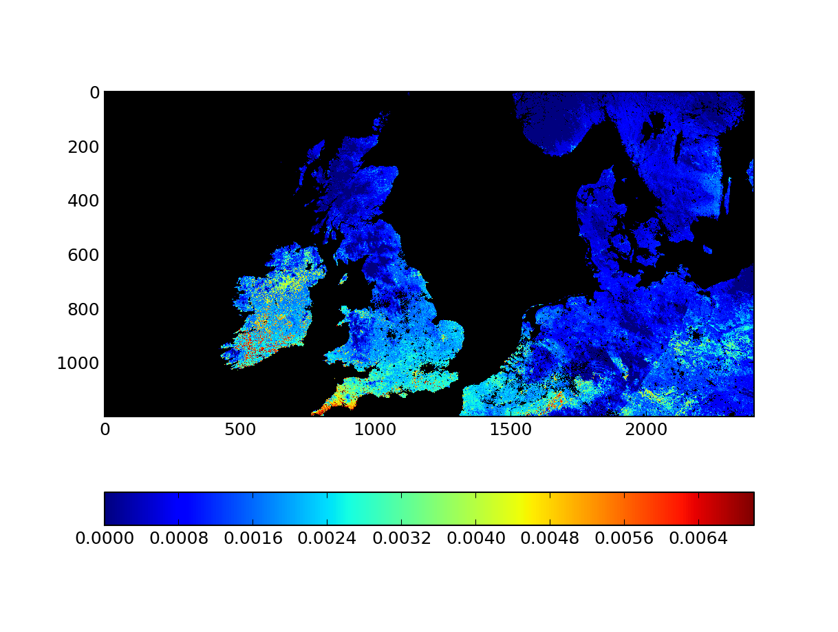
Note that we have escaped the GDAL filenames here. You can check the output file, mosaic_sinu.vrt, with gdalinfo and satisfiy yourself that it makes sense: We have just stitched two adjacent tiles into a single dataset. We can have a look at the result with Python (who can read the VRT files just fine!):
import numpy as np
import matplotlib.pyplot as plt
from osgeo import gdal

g = gdal.Open ( "mosaic_sinu.vrt" ) # Open file
data = g.ReadAsArray() # Read contents
mdata = np.ma.array ( data, mask=data>30000 ) # Mask data
cmap = plt.cm.jet # Set colormap
cmap.set_bad ( 'k' ) # Set masked values to black
# Next line scales the GPP data by 0.0001 to get the right units
# and plots it.
plt.imshow ( mdata*0.0001, interpolation='nearest', vmax=0.007, cmap=cmap)
plt.colorbar ( orientation='horizontal' )
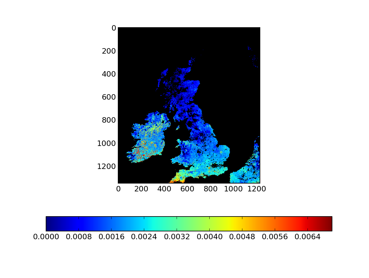
Let's say we want to use the Ordnance Survey Projection for the UK. In this webpage, the reader is pointed to a projection definition that GDAL will understand, EPSG:27700. We can now feed this to gdalwarp and have virtually projected dataset!
gdalwarp -of VRT -t_srs "EPSG:27700" mosaic_sinu.vrt mosaic.vrt
This is nice, but it applies the projection to most of the Netherlands, and southern Scandinavia. If we just want to crop the UK and Ireland, we can do that as well. Say we want to cut out the box that extends from longitudes -14 to 5 and latitudes 50 to 61. Using gdaltransform
.. code-block: bash
# Upper left corner echo -14 61 | gdaltransform -s_srs "EPSG:4326" -t_srs "EPSG:27700" -246410.748854375 1294822.36205397 -54.5953653845936 # Lower right corner echo 5 50 | gdaltransform -s_srs "EPSG:4326" -t_srs "EPSG:27700" 901561.991813587 34610.1630877961 -35.8900839695707
We use gdal_translate to crop the region of interest
gdal_translate -of VRT -projwin -246410.748854375 1294822.36205397 901561.991813587 34610.1630877961 mosaic.vrt mosaic_cropped.vrt
At this stage, we have the output that we want for a given date. Let's put this together for a whole year.
All dates
We need a script that automates the previous task. Here:
#!/bin/bash

tile1=$1
tile2=$2
year=$3

# First grab the available dates for one tile
hdf_tile1=(`ls MOD17A2.A${year}*${tile1}*.hdf`)
\rm -rf file_list.txt
# Loop through datasets in time...
for t1 in "${hdf_tile1[@]}"
do

     t2=`echo $t1| awk -F"."  -v other_tile=$tile2 \
         '{printf( "%s.%s.%s.*\n",  $1,$2,other_tile)}'`
     t2=`ls $t2`
     output_fname=`echo $t1| awk -F"."  '{printf( "%s.%s\n",  $1,$2)}'`
     echo ${t1} ${t2} ${output_fname}
     gdalbuildvrt ${output_fname}_mosaic_sinu.vrt \
         'HDF4_EOS:EOS_GRID:"'${t1}'":MOD_Grid_MOD17A2:Gpp_1km' \
         'HDF4_EOS:EOS_GRID:"'${t2}'":MOD_Grid_MOD17A2:Gpp_1km'
      gdalwarp -of VRT -t_srs "EPSG:27700" ${output_fname}_mosaic_sinu.vrt \
               ${output_fname}_mosaic.vrt
      gdal_translate -of VRT \
          -projwin -246410.748854375 1294822.36205397 901561.991813587 34610.1630877961 \
          ${output_fname}_mosaic.vrt ${output_fname}.vrt
      echo ${output_fname}.vrt >> file_list.txt

done
We run the script for each year as
stitch_files.sh h18v03 h17v03 2004
Putting all that together
In the previous script, a file called file_list.txt holds the name of all the output VRT files. We will now create a multiband VRT file using all the reprojected and cropped files, and then convert the VRT file to a GeoTIFF file:
gdalbuildvrt -separate -input_file_list file_list.txt MOD17A2.2004.vrt
gdal_translate -of GTiff -co "COMPRESS=LZW" -co "TILED=YES" MOD17A2.2004.vrt MOD17A2.2004.tif
At this stage, we can have a look at MOD17A2.2004.tif with e.g. gdalinfo or something.