How to extract spectra from image data using ground truth vector data
Supervised classification of EO data uses a set of samples from known patterns (usually reflectance spectra) to decide whether a given pattern belongs to one class or another. In landcover applications, one goes to the field, and observes that a given location is indeed class $\omega_c$. These ground observations usually find their ways into a vector dataset, and they can be used to extract the relevant pixels from satellite data in raster formats. Let's see how this is done. I'm assuming that I have two sets of files:
- 409_QB05_1merg.shp
- a shapefile, where each feature is encoded as a multipolygon,
- ortodvd7_402_multiespectral.tif
- a raster file with a few bands (some multispectral dataset).
Let's first note the extent and resolution of the GeoTIFF file with gdalinfo
gdalinfo ortodvd7_402_multiespectral.tif
Driver: GTiff/GeoTIFF
Files: ortodvd7_402_multiespectral.tif
       ortodvd7_402_multiespectral.aux
       ortodvd7_402_multiespectral.rrd
       ortodvd7_402_multiespectral.tfw
Size is 6380, 5668
Coordinate System is:
PROJCS["UTM Zone 30N",
    GEOGCS["European_1950_Portugal_Spain",
        DATUM["European_1950_Portugal_Spain",
            SPHEROID["International 1909",6378388,297.0000000284015]],
        PRIMEM["Greenwich",0],
        UNIT["degree",0.0174532925199433]],
    PROJECTION["Transverse_Mercator"],
    PARAMETER["latitude_of_origin",0],
    PARAMETER["central_meridian",-3],
    PARAMETER["scale_factor",0.9996],
    PARAMETER["false_easting",500000],
    PARAMETER["false_northing",0],
    UNIT["metre",1,
        AUTHORITY["EPSG","9001"]]]
Origin = (143110.649999999994179,4132515.350000000093132)
Pixel Size = (2.700000000000000,-2.700000000000000)
Metadata:
  TIFFTAG_SOFTWARE=ERDAS IMAGINE
  TIFFTAG_XRESOLUTION=1
  TIFFTAG_YRESOLUTION=1
  TIFFTAG_RESOLUTIONUNIT=1 (unitless)
  AREA_OR_POINT=Area
Image Structure Metadata:
  INTERLEAVE=PIXEL
Corner Coordinates:
Upper Left  (  143110.650, 4132515.350) (  7d 1'27.45"W, 37d16'12.83"N)
Lower Left  (  143110.650, 4117211.750) (  7d 1' 1.14"W, 37d 7'57.46"N)
Upper Right (  160336.650, 4132515.350) (  6d49'49.65"W, 37d16'36.02"N)
Lower Right (  160336.650, 4117211.750) (  6d49'24.59"W, 37d 8'20.53"N)
Center      (  151723.650, 4124863.550) (  6d55'25.71"W, 37d12'16.85"N)
Band 1 Block=6380x8 Type=UInt16, ColorInterp=Gray
  Min=0.000 Max=1599.000
  Minimum=0.000, Maximum=1599.000, Mean=128.363, StdDev=89.004
  Overviews: 1595x1417, 798x709, 399x355, 200x178, 100x89, 50x45
  Metadata:
    STATISTICS_MINIMUM=0
    STATISTICS_MAXIMUM=1599
    STATISTICS_MEAN=128.36316119423
    STATISTICS_MEDIAN=3.2133151845658e-234
    STATISTICS_MODE=4.4506188044836e-308
    STATISTICS_STDDEV=89.003854388224
    LAYER_TYPE=athematic
Band 2 Block=6380x8 Type=UInt16, ColorInterp=Undefined
  Min=0.000 Max=2047.000
  Minimum=0.000, Maximum=2047.000, Mean=180.116, StdDev=141.805
  Overviews: 1595x1417, 798x709, 399x355, 200x178, 100x89, 50x45
  Metadata:
    STATISTICS_MINIMUM=0
    STATISTICS_MAXIMUM=2047
    STATISTICS_MEAN=180.11620984994
    STATISTICS_MEDIAN=3.2133151845658e-234
    STATISTICS_MODE=4.4506188044836e-308
    STATISTICS_STDDEV=141.80527606593
    LAYER_TYPE=athematic
Band 3 Block=6380x8 Type=UInt16, ColorInterp=Undefined
  Min=0.000 Max=2047.000
  Minimum=0.000, Maximum=2047.000, Mean=116.447, StdDev=116.221
  Overviews: 1595x1417, 798x709, 399x355, 200x178, 100x89, 50x45
  Metadata:
    STATISTICS_MINIMUM=0
    STATISTICS_MAXIMUM=2047
    STATISTICS_MEAN=116.44734908401
    STATISTICS_MEDIAN=3.2133151845658e-234
    STATISTICS_MODE=4.4506188044836e-308
    STATISTICS_STDDEV=116.2210329906
    LAYER_TYPE=athematic
Band 4 Block=6380x8 Type=UInt16, ColorInterp=Undefined
  Min=0.000 Max=2047.000
  Minimum=0.000, Maximum=2047.000, Mean=171.386, StdDev=166.748
  Overviews: 1595x1417, 798x709, 399x355, 200x178, 100x89, 50x45
  Metadata:
    STATISTICS_MINIMUM=0
    STATISTICS_MAXIMUM=2047
    STATISTICS_MEAN=171.38578244359
    STATISTICS_MEDIAN=5.4413901556992e-227
    STATISTICS_MODE=1.4092176116584e-315
    STATISTICS_STDDEV=166.74819006626
    LAYER_TYPE=athematic
We can see the four bands (R, G, B and NIR), their statistics in terms of DN, as well as the extent, resolution and rows & columns. Now, let's have a look at the Shapefile with ogrinfo
ogrinfo -al -so 409_QB05_1merg.shp
INFO: Open of `409_QB05_1merg.shp'
      using driver `ESRI Shapefile' successful.

      Layer name: 409_QB05_1merg
      Geometry: Polygon
      Feature Count: 16
      Extent: (146113.385068, 4119178.250911) - (153213.897681, 4132145.765108)
      Layer SRS WKT:
      (unknown)
The shapefile doesn't contain a projection, but it would appear that it belongs with the image. We also note that there is no layer, but in fact, the 16 features are the different classes. As in a previous entry, we can create a raster mask that will allow us to select the spectra in the multispectral dataset using gdal_rasterize
gdal_rasterize -of GTiff  -a_nodata 0 -co "COMPRESS=LZW" -a FID  \
    -sql "select FID, * from '409_QB05_1merg'" -ot Byte \
    -te 143110.650 4117211.750 160336.650 4132515.350 \
    -ts 6380 5668 -a_srs "EPSG:23030" 409_QB05_1merg.shp mascara.tif
I have set the projection to be UTM 30N/ED50 (same as in the geotiff), the no data value to be 0, and the data type to be byte (this is to save memory: it's pointless using integers when our mask will only go from 0 to 16). I have also set GeoTIFF options to compress the data, so that the mask file is a meagre ~840kb of data. We can also plot the result
import numpy as np
import matplotlib.pyplot as plt
from osgeo import gdal_rasterize

g = gdal.Open ( "mascara.tif" )
m = g.ReadAsArray()
mm = np.ma.array ( m, mask=(m==0) )
g = gdal.Open("ortodvd7_402_multiespectral.tif")
data = g.ReadAsArray()
ss =  np.rollaxis(data[:3, ::10, ::10], 0, 3)
plt.imshow ( ss/822., interpolation='nearest', \
        extent=(0, 6380, 0, 5668) )
plt.hold ( True )
plt.imshow ( mm, interpolation='nearest',  vmin=1, vmax=16,\
        extent=(0, 6380, 0, 5668), cmap=plt.cm.Reds)
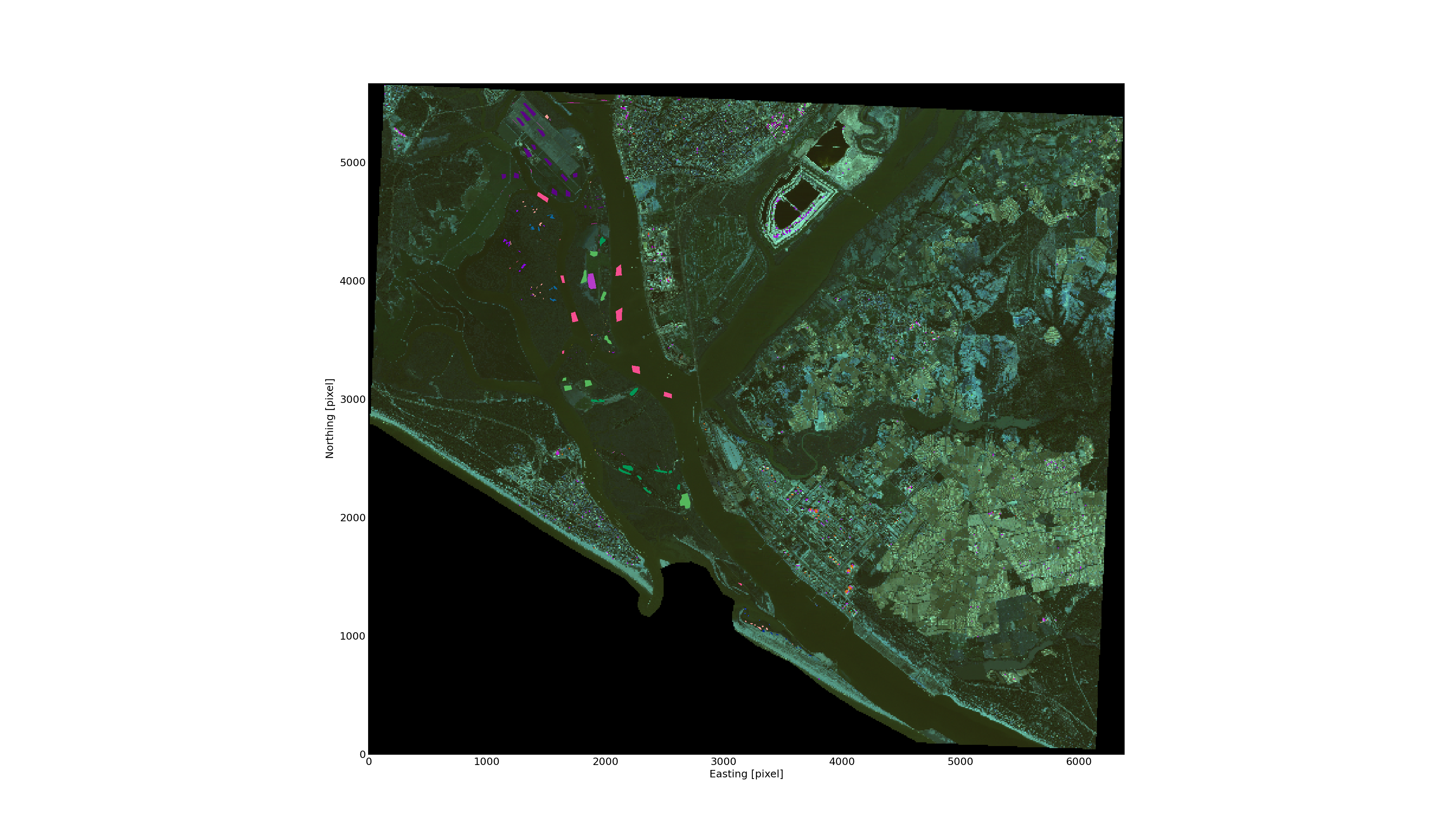
The selected polygons on top of the raster data using different colours.
import numpy as np
import matplotlib.pyplot as plt
from osgeo import gdal_rasterize

g = gdal.Open ( "mascara.tif" )
m = g.ReadAsArray()
mm = np.ma.array ( m, mask=(m==0) )
g = gdal.Open("ortodvd7_402_multiespectral.tif")
data = g.ReadAsArray()
spectra = np.c_[ 1*np.ones(np.sum(m==1)), data[:, m==1].T]
for i in xrange( 2, 17 ):
    spectra = np.r_ [ spectra, np.c_[ i*np.ones(np.sum(m==i)), \
            data[:, m==i].T] ]

# Plot some classes...
fig = plt.figure()
ax = fig.add_subplot(111, projection='3d')
color=['r', 'g', 'b', 'y', 'k' ]
for i in xrange(2, 6):
   isel = spectra[:,0] == i
   ax.scatter ( spectra[isel, 2], spectra[isel, 3], \
           spectra[isel,4], marker='o', c=color[i-2] )
# Save the spectra as a text file
np.savetxt("spectra.txt", spectra, fmt="%8g")
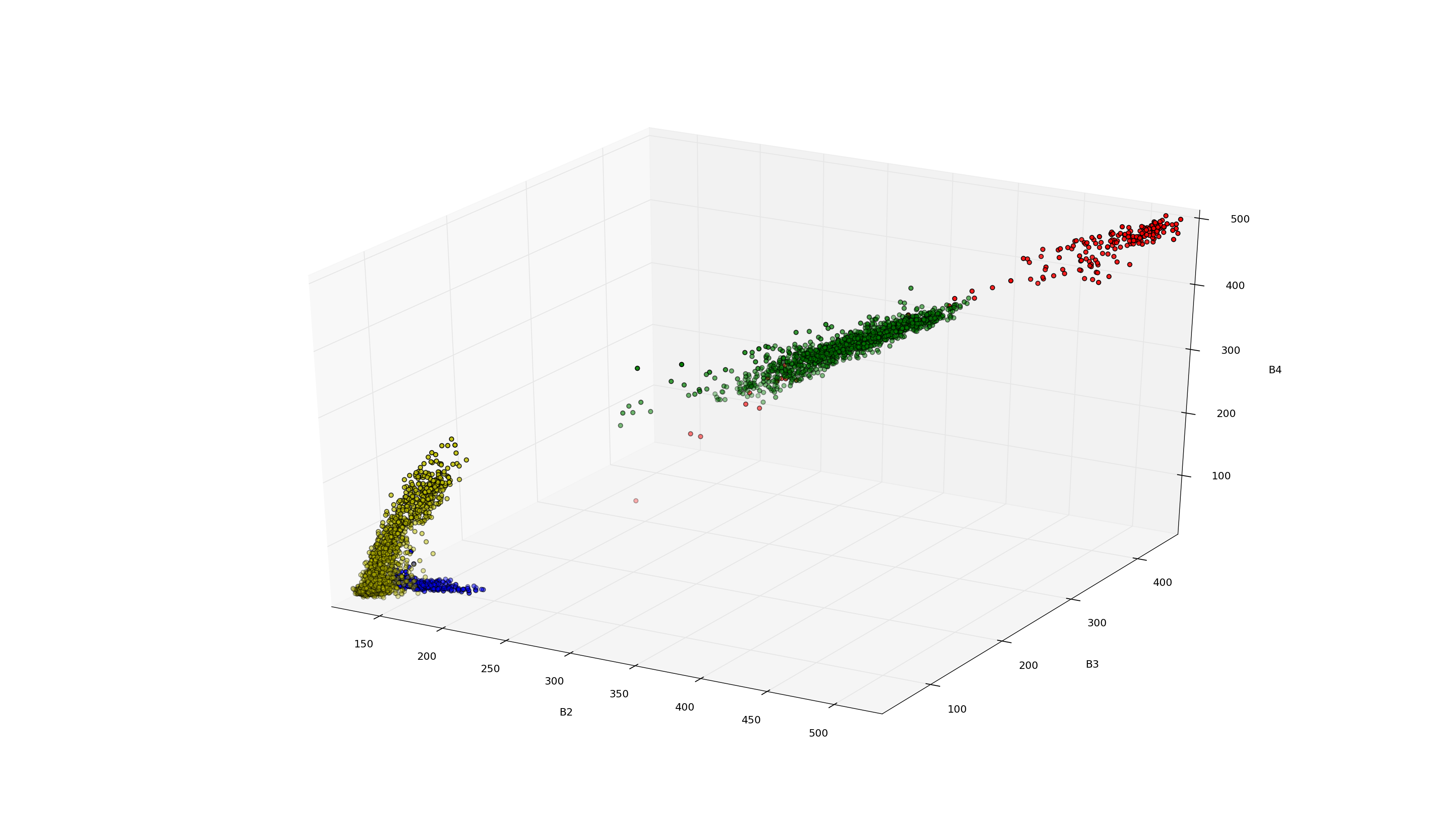
The extracted pixels for classes 2 to 5 over feature dimensions 2, 3 and 4. Note how the different classes can be separated.