Starting to use Python to work with geospatial data

Start by launching in a console window the ipython interpreter. It is useful to launch ipython with the -pylab option, as this will load a number of useful modules (numpy, scipy and matplotlib), saving you the hassle of loading them yourself. The documentation for ipython is quite extensive.

$ ipython -pylab
WARNING: `-pylab` flag has been deprecated.
Use `--pylab` instead, or `--pylab=foo` to specify a backend.
Enthought Python Distribution -- www.enthought.com

Python 2.7.2 |EPD 7.1-2 (64-bit)| (default, Jul  3 2011, 15:17:51)
Type "copyright", "credits" or "license" for more information.

IPython 0.11 -- An enhanced Interactive Python.
?         -> Introduction and overview of IPython's features.
%quickref -> Quick reference.
help      -> Python's own help system.
object?   -> Details about 'object', use 'object??' for extra details.

Welcome to pylab, a matplotlib-based Python environment [backend: WXAgg].
For more information, type 'help(pylab)'.

In [1]:

You can try and type python commands here. However, in order to use the GDAL bindings, we need to first import the osgeo.gdal module. Also, you can check the documentation by typing help (gdal). The first thing to do is to read a file into python. We shall use a MODIS HDF file, that you can find on the system in /data/geospatial_10/ucfajlg/MOD12/MCD12Q1.A2005001.h17v03.005.2008310174635.hdf. Since HDF files have subdatasets, we’ll open the HDF file, examine the subdatasets and then load the subdataset we are interested in (to GDAL, a subdataset is a normal file, albeit one with a peculiar filename). So we create a GDAL object by using the gdal.Open function. This function requires a filename (see line[2] below). We then use the GetSubDatasets() method on the GDAL object to list the subdatasets, as well as their descriptions. Note that this is a list, where each element (each dataset) is a tuple. The first element of the tuple is the GDAL subdataset “filename”. It includes the real filename, as well as the particular subdataset. To save typing, you can store the return of GetSubDatasets() into a variable and refer to the filename for the Land_Cover_Type_5 dataset by inspecting element [4][0] of the variable where you stored the subdatasets. But for now, just load data for Land_Cover_Type_1 in a variable called lc_fich

In [1]: from osgeo import gdal

In [2]: gdal_dataset = gdal.Open ("/data/geospatial_10/ucfajlg/MOD12/MCD12Q1.A2005001.h17v03.005.2008310174635.hdf")

In [3]: gdal_dataset.GetSubDatasets()
Out[3]:
[('HDF4_EOS:EOS_GRID:"/data/geospatial_10/ucfajlg/MOD12/MCD12Q1.A2005001.h17v03.005.2008310174635.hdf":MOD12Q1:Land_Cover_Type_1',
'[2400x2400] Land_Cover_Type_1 MOD12Q1 (8-bit unsigned integer)'),
('HDF4_EOS:EOS_GRID:"/data/geospatial_10/ucfajlg/MOD12/MCD12Q1.A2005001.h17v03.005.2008310174635.hdf":MOD12Q1:Land_Cover_Type_2',
'[2400x2400] Land_Cover_Type_2 MOD12Q1 (8-bit unsigned integer)'),
('HDF4_EOS:EOS_GRID:"/data/geospatial_10/ucfajlg/MOD12/MCD12Q1.A2005001.h17v03.005.2008310174635.hdf":MOD12Q1:Land_Cover_Type_3',
'[2400x2400] Land_Cover_Type_3 MOD12Q1 (8-bit unsigned integer)'),
('HDF4_EOS:EOS_GRID:"/data/geospatial_10/ucfajlg/MOD12/MCD12Q1.A2005001.h17v03.005.2008310174635.hdf":MOD12Q1:Land_Cover_Type_4',
'[2400x2400] Land_Cover_Type_4 MOD12Q1 (8-bit unsigned integer)'),
('HDF4_EOS:EOS_GRID:"/data/geospatial_10/ucfajlg/MOD12/MCD12Q1.A2005001.h17v03.005.2008310174635.hdf":MOD12Q1:Land_Cover_Type_5',
'[2400x2400] Land_Cover_Type_5 MOD12Q1 (8-bit unsigned integer)'),
('HDF4_EOS:EOS_GRID:"/data/geospatial_10/ucfajlg/MOD12/MCD12Q1.A2005001.h17v03.005.2008310174635.hdf":MOD12Q1:Land_Cover_Type_1_Assessment',
'[2400x2400] Land_Cover_Type_1_Assessment MOD12Q1 (8-bit unsigned integer)'),
('HDF4_EOS:EOS_GRID:"/data/geospatial_10/ucfajlg/MOD12/MCD12Q1.A2005001.h17v03.005.2008310174635.hdf":MOD12Q1:Land_Cover_Type_2_Assessment',
'[2400x2400] Land_Cover_Type_2_Assessment MOD12Q1 (8-bit unsigned integer)'),
('HDF4_EOS:EOS_GRID:"/data/geospatial_10/ucfajlg/MOD12/MCD12Q1.A2005001.h17v03.005.2008310174635.hdf":MOD12Q1:Land_Cover_Type_3_Assessment',
'[2400x2400] Land_Cover_Type_3_Assessment MOD12Q1 (8-bit unsigned integer)'),
('HDF4_EOS:EOS_GRID:"/data/geospatial_10/ucfajlg/MOD12/MCD12Q1.A2005001.h17v03.005.2008310174635.hdf":MOD12Q1:Land_Cover_Type_4_Assessment',
'[2400x2400] Land_Cover_Type_4_Assessment MOD12Q1 (8-bit unsigned integer)'),
('HDF4_EOS:EOS_GRID:"/data/geospatial_10/ucfajlg/MOD12/MCD12Q1.A2005001.h17v03.005.2008310174635.hdf":MOD12Q1:Land_Cover_Type_5_Assessment',
'[2400x2400] Land_Cover_Type_5_Assessment MOD12Q1 (8-bit unsigned integer)'),
('HDF4_EOS:EOS_GRID:"/data/geospatial_10/ucfajlg/MOD12/MCD12Q1.A2005001.h17v03.005.2008310174635.hdf":MOD12Q1:Land_Cover_Type_QC',
'[1x2400x2400] Land_Cover_Type_QC MOD12Q1 (8-bit unsigned integer)'),
('HDF4_EOS:EOS_GRID:"/data/geospatial_10/ucfajlg/MOD12/MCD12Q1.A2005001.h17v03.005.2008310174635.hdf":MOD12Q1:Land_Cover_Type_1_Secondary',
'[2400x2400] Land_Cover_Type_1_Secondary MOD12Q1 (8-bit unsigned integer)'),
('HDF4_EOS:EOS_GRID:"/data/geospatial_10/ucfajlg/MOD12/MCD12Q1.A2005001.h17v03.005.2008310174635.hdf":MOD12Q1:Land_Cover_Type_1_Secondary_Percent',
'[2400x2400] Land_Cover_Type_1_Secondary_Percent MOD12Q1 (8-bit unsigned integer)'),
('HDF4_EOS:EOS_GRID:"/data/geospatial_10/ucfajlg/MOD12/MCD12Q1.A2005001.h17v03.005.2008310174635.hdf":MOD12Q1:LC_Property_1',
'[2400x2400] LC_Property_1 MOD12Q1 (8-bit unsigned integer)'),
('HDF4_EOS:EOS_GRID:"/data/geospatial_10/ucfajlg/MOD12/MCD12Q1.A2005001.h17v03.005.2008310174635.hdf":MOD12Q1:LC_Property_2',
'[2400x2400] LC_Property_2 MOD12Q1 (8-bit unsigned integer)'),
('HDF4_EOS:EOS_GRID:"/data/geospatial_10/ucfajlg/MOD12/MCD12Q1.A2005001.h17v03.005.2008310174635.hdf":MOD12Q1:LC_Property_3',
'[2400x2400] LC_Property_3 MOD12Q1 (8-bit unsigned integer)')]

In [4]: lc_data = gdal.Open ( 'HDF4_EOS:EOS_GRID:"/data/geospatial_10/ucfajlg/MOD12/MCD12Q1.A2005001.h17v03.005.2008310174635.hdf":MOD12Q1:Land_Cover_Type_1' )

In ipython, you can use tab-completion or the ? symbol to explore objects. It will report methods associated with the object in question. Use this facility to list the methods available for lc_data. Some of the most important methods are

GetGeoTransform ()

This method returns the 6-element geotransform described in the previous section.

GetMetadata ()

This method returns a dictionary with the metadata items.

GetRasterBand ( band )

This method selects a band (and returns a pointer to it). In GDAL, band numbers start at 1, rather than 0.

RasterCount

The number of bands (will be one or more).

RasterXSize

The size in pixels of the dataset in the horizontal (x) direction

RasterYSize

The size in pixels of the dataset in the vertical (y) direction

GetProjectionRef ()

Returns the projection reference (as a WKT string)

ReadAsArray ()

Reads the whole dataset as a numpy array of size ( RasterCount, RasterXSize, RasterYSize ). While very convenient, be wary that some datasets are very large, and this will read all of it into memory.

ReadRaster ()

An efficient way of reading a chunk of the dataset.

You can use the above methods to examine the dataset. Take a minute to look at the geotransfrom, metadata, and size of the dataset. Think about the memory you will be using just to store it in memory. To actually load the data into an array, use the ReadAsArray method. Also, let’s just check the size of the dataset in Mb, and some statistics about the data

In [15]: lc = lc_data.ReadAsArray()

In [16]: (lc.nbytes/(8*1024*1024.))
Out[16]: 0.6866455078125

In [20]: (lc.min(), lc.max(), lc.mean(), lc.std())
Out[20]: (0, 16, 2.2486869791666666, 4.2774078780394431)

In [22]: passer = np.logical_and ( lc > 0, lc <= 16)

In [23]: (lc[passer].min(), lc[passer].max(), lc[passer].mean(), lc[passer].std())
Out[23]: (1, 16, 9.4393890256958137, 2.9877779088248566)

When we exclude the ocean (landcover value of 0), and select only the pixels where the landcover is between 1 and 16 (inclusive both), we see that the mean and standard deviation of the dataset change dramatically. We are using a slice of the data from the logical array defined as passer. This provides a view of the original array: it doesn’t modify it, but only returns an array where the condition is true.

Plotting the data

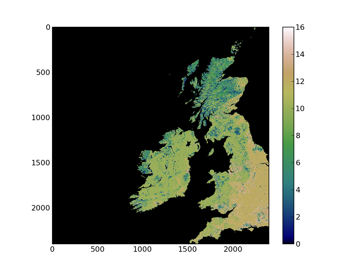
Let’s quickly have a look at the data in lc. Since it is just an array, we can plot it directly with matplotlib:

In [29]: plt.imshow ( lc, interpolation='nearest', vmin=0, cmap=plt.cm.gist_earth)
Out[29]: <matplotlib.image.AxesImage at 0xccc0650>

In [30]: plt.colorbar()
Out[30]: <matplotlib.colorbar.Colorbar instance at 0xcce9560>

The previous code snippet uses imshow. The first argument is the array (it has to be a 2D array), the second named argument (interpolation='nearest') tells matplotlib not to interpolate between pixels. vmin=0 gives the lowest value of the array that will be mapped to the lowest value of the colormap (in this case 0). cmap selects a matplotlib colormap. You can see what colormaps are available in this page. Finally, we add a colorbar. These commands provide the following visualisation