Finding things in raster files

The simplest scenario

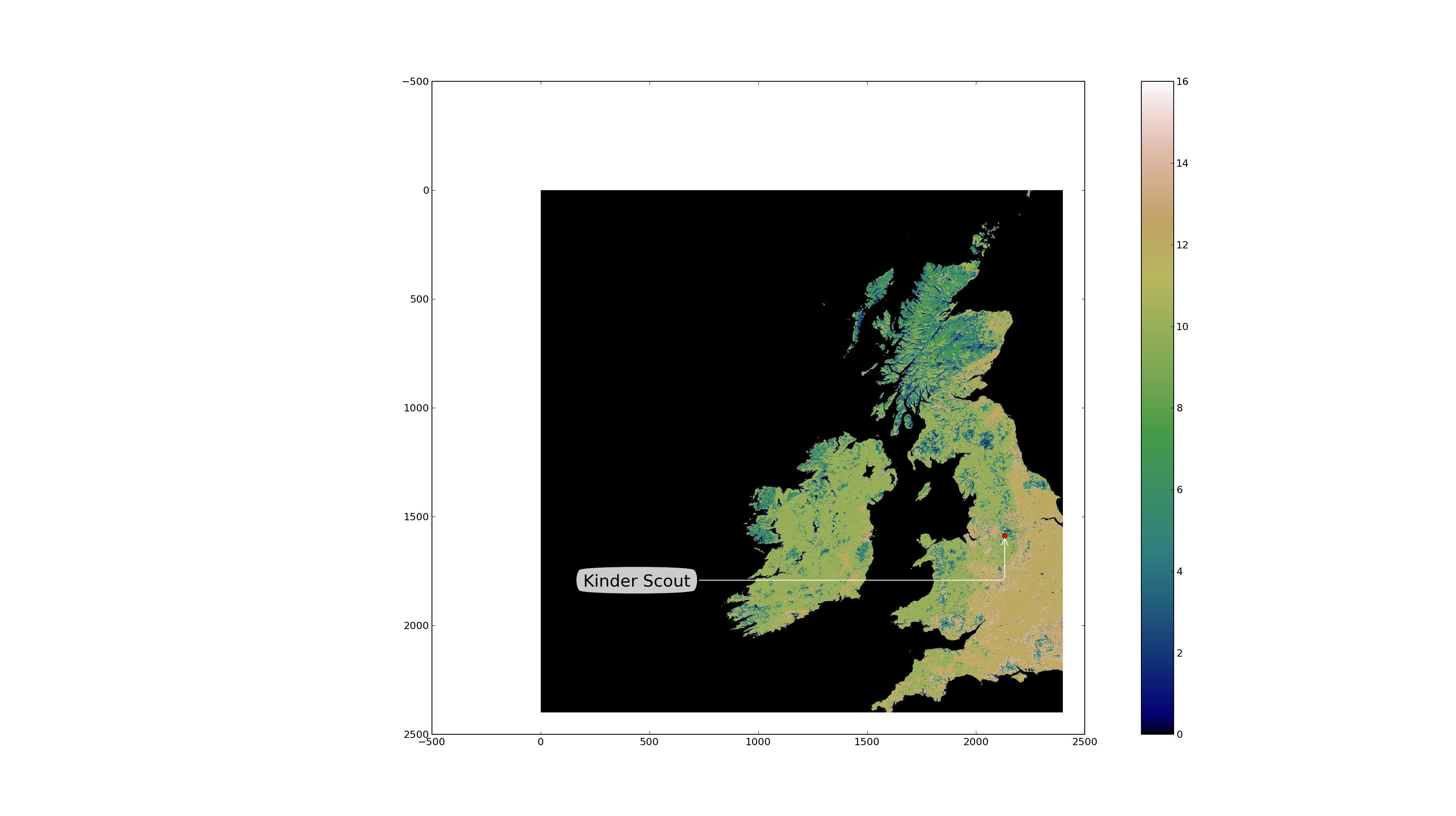
The simplest scenario is to find a pixel when we know the coordinates of that pixel in the same projection as the geospatial dataset. This is farily common when working with high resolution data, usually in UTM coordinates, or when working with unprojected global datasets on a longitude/latitude grid. To find the pixel locations of coordinates, we need to use the geotransform. Assume we are interested in locating Kinder Scout, a moorland in the Peak District National Park. Its coordinates are 1.871417W, 53.384726N. In the MODIS integerised sinusoidal projection, the coordinates [1] are (-124114.3, 5936117.4). Let’s calculate what pixel location is that, and plot a callbox in our map

In [50]: geot = lc_data.GetGeoTransform()

In [52]: geot
Out[52]: (-1111950.519667, 463.3127165279167, 0.0, 6671703.118, \
            0.0, -463.3127165279165)

In [53]: # See the nominal resolution for MODIS 0.5km data, 463 in x \
         #and y. Note the -ve sign in the y as we start at the UL corner
In [54]: pixel_x = (-124114.3 - geot[0])/geot[1] \
        # The difference in distance between the UL corner (geot[0] \
        #and point of interest. Scaled by geot[1] to get pixel number

In [55]: pixel_x
Out[55]: 2132.115490094644 # A real number, not an integer!

In [59]: pixel_y = (5936117.4 - geot[3])/(geot[5]) # Like for pixel_x, \
        #but in vertical direction. Note the different elements of geot \
        #being used

In [60]: pixel_y
Out[60]: 1587.66572070913 # Quick check: both pixel_x and pixel_y \
           # are >=0 and pixel_x <= lc_data.RasterXSize and \
           # pixel_y <= lc_data.RasterYSize

In [79]: plt.plot ( pixel_x, pixel_y, 'ro') # Add a red dot
Out[79]: [<matplotlib.lines.Line2D at 0x1064e2d0>]

In [80]: plt.annotate('Kinder Scout', xy=(pixel_x, pixel_y),  \
        xycoords='data', xytext=(-500, -60), \
        textcoords='offset points',  size=20, \
        bbox=dict(boxstyle="round4,pad=.5", fc="0.8"), \
        arrowprops=dict(arrowstyle="->", \
        connectionstyle="angle,angleA=0,angleB=-90,rad=10", \
        color='w'), )
Out[80]: <matplotlib.text.Annotation at 0x10653090>

The last line that annotates the location of Kinder Scout is quite convoluted (see documentation on annotate in here. Most of the command is taken from the examples there), but the final output is this:

Try it out on some other places

Find the longitude and latitude of some places of interest in the British isles (West of Greenwich!) and using the MODLAND MODIS tile calculator and the geotransform, repeat the above experiment. Note that the MODIS calculator calculates both the projected coordinates in the MODIS sinusoidal projection, as well as the pixel number, so it is a helpful way to check whether you got the right result.

Park name	Longitude [deg]	Latitude [deg]
Dartmoor national park	-3.904	50.58
New forest national park	-1.595	50.86
Exmoor national park	-3.651	51.14
Pembrokeshire coast national park	-4.694	51.64
Brecon beacons national park	-3.432	51.88
Pembrokeshire coast national park	-4.79	51.99
Norfolk and suffolk broads	1.569	52.62
Snowdonia national park	-3.898	52.9
Peak district national park	-1.802	53.3
Yorkshire dales national park	-2.157	54.23
North yorkshire moors national park	-0.8855	54.37
Lake district national park	-3.084	54.47
Galloway forest park	-4.171	54.87
Galloway forest park	-4.191	55.18
Galloway forest park	-4.379	55.28
Northumberland national park	-2.228	55.28
Loch lomond & the trossachs national park	-4.593	56.24
Tay forest park	-4.025	56.59
Cairngorms national park	-3.545	57.08

Reprojecting from python

The most general situation is that the points of interest and the geospatial dataset have different projections. For example, GPS receivers often quote WGS84 coordinates (and so does Google maps!). We shall see how to use GDAL to project data. The basics of this require the import of the osr module, and defining two SpatialReference object, one for the source projection and one for the destination projection. In GDAL, there are many different ways of defining projections. We’ve seen the EPSG codes, but we can also use the widely availabe Proj4 format, WKT, ESRI, etc. You can use spatialreference.org to conveniently search for projections in a multitude of GDAL-useable formats. Once the projections are in place, one needs to define a CoordinateTransformation object. This object takes the two projection objects, and will have a method called TransformPoint that will transform a set of coordinates for you.

Let’s demonstrate these concepts with a script. This script first sets up the WGS84 and MODIS sinusoidal projections. It uses them to create a CoordinateTransformation object. Once this is done, it loops over the table presented above, extracts the longitude and latitude, and feeds these to the transformation method. Note that this method returns three numbers (x,y,z), as there could be a shift of height by changing the geoid or the datum.

#!/usr/bin/env python

from osgeo import ogr
from osgeo import osr
"""
SYNOPSIS

project_points.py

DESCRIPTION

A script to convert longitude latitude coordinates in WGS84 to the MODIS 
sinusoidal projection using GDAL. Currently it uses a big string, but can you 
modify it to take data in a file, or make it into a function?

AUTHOR

Jose Gomez-Dans <j.gomez-dans@geog.ucl.ac.uk>

LICENSE

This script is in the public domain, free from copyrights or restrictions.

VERSION

1.0
"""



# The next line defines the data as a string
# as would be for example if read from a file etc.
park_data = """Dartmoor national park,             -3.904,              50.58
New forest national park,             -1.595,              50.86
Exmoor national park,             -3.651,              51.14
Pembrokeshire coast national park,             -4.694,              51.64
Brecon beacons national park,             -3.432,              51.88
Pembrokeshire coast national park,              -4.79,              51.99
Norfolk and suffolk broads,              1.569,              52.62
Snowdonia national park,             -3.898,               52.9
Peak district national park,             -1.802,               53.3
Yorkshire dales national park,             -2.157,              54.23
North yorkshire moors national park,            -0.8855,              54.37
Lake district national park,             -3.084,              54.47
Galloway forest park,             -4.171,              54.87
Galloway forest park,             -4.191,              55.18
Galloway forest park,             -4.379,              55.28
Northumberland national park,             -2.228,              55.28
Loch lomond & the trossachs national park,            -4.593,              56.24
Tay forest park,             -4.025,              56.59
Cairngorms national park,             -3.545,              57.08"""

# Define the source projection, WGS84 lat/lon. 
wgs84 = osr.SpatialReference( ) # Define a SpatialReference object
wgs84.ImportFromEPSG( 4326 ) # And set it to WGS84 using the EPSG code

# Now for the target projection, MODIS sinusoidal
modis_sinu = osr.SpatialReference() # define the SpatialReference object
# In this case, we get the projection from a Proj4 string
modis_sinu.ImportFromProj4 ( \
                "+proj=sinu +R=6371007.181 +nadgrids=@null +wktext")

# Now, we define a coordinate transformtion object, *from* wgs84 *to* modis_sinu
tx = osr.CoordinateTransformation( wgs84, modis_sinu )
# We loop over the lines of park_data, 
#         using the split method to split by newline characters
for linea in park_data.split( "\n" ):
    # Split linea by spacing
    park_name, lon, lat = linea.split(",")
    # Convert longitude and latitude values to floats
    # they are strings at the moment
    lon = float ( lon )
    lat = float ( lat )
    # Actually do the transformation using the TransformPoint method
    modis_x, modis_y, modis_z = tx.TransformPoint ( lon, lat )
    # Print out
    print park_name, lon, lat, modis_x, modis_y

The sample ouput (park name, longitude, latitude, MODIS x coordinate and MODIS y coordinate) is

Dartmoor national park -3.904 50.58 -275657.072566 5624245.72898
New forest national park -1.595 50.86 -111950.267741 5655380.34353
Exmoor national park -3.651 51.14 -254715.497137 5686514.95809
[...]

Some more examples

1. Modify the script above, try convert the location of the national parks and plot them eg as a circle to the MODIS land cover image. Think about how you deal with parks that may be outside the area covered by the image.
2. Try to convert the WGS84 data into a different coordinate system, and then convert these new coordinates back into WGS84.

Saving data

Up to now, we have covered how to read data into numpy arrays. These arrays can be used to visualise the data, or to carry further processig on them. For example, you could write a simple function to read red and near-infrarred reflectances and calculate a vegetation index [2] quite simply by

def calculate_ndvi ( red_filename, nir_filename ):
    """
    A function to calculate the Normalised Difference Vegetation Index
    from red and near infrarred reflectances. The reflectance data ought to
    be present on two different files, specified by the varaibles 
    `red_filename` and `nir_filename`. The file format ought to be
    recognised by GDAL
    """
    from osgeo import gdal
    g = gdal.Open ( red_filename )
    red = g.ReadAsArray()
    g = gdal.Open ( nir_filename )
    nir = g.ReadAsArray()
    ndvi = ( 1.*nir - red ) / ( 1.*nir + red )
    return ndvi

In the previous example, we make sure that the variables are made real numbers by multiplying them by a constant 1.0. Now, this is easy and useful, but how do you save this data so you can re-use it? As we’ve seen above, a GDAL file consists of the data, a geotransform and a projection reference. Addtionally, we need to define what output format we want. So far, we have the data (the output of calculate_ndvi). We do not have the geotransform or the spatial reference, but these can probably be gleaned from the reflectance datasets. In fact, if these are different for the red and nir bands (geolocation and projection reference), then the user should be warned of this, as it is likely that the datasets are different.

def save_raster ( output_name, raster_data, dataset, driver="GTiff" ):
    """
    A function to save a 1-band raster using GDAL to the file indicated
    by ``output_name``. It requires a GDAL-accesible dataset to collect 
    the projection and geotransform.
    """
    # Open the reference dataset
    g = gdal.Open ( dataset )
    # Get the Geotransform vector
    geo_transform = g.GetGeoTransform ()
    x_size = g.RasterXSize # Raster xsize
    y_size = g.RasterYSize # Raster ysize
    srs = g.GetProjectionRef () # Projection
    # Need a driver object. By default, we use GeoTIFF
    driver = gdal.GetDriverByName ( driver )
    dataset_out = driver.Create ( output_name, x_size, y_size, 1, \
            gdal.GDT_Float32 )
    dataset_out.SetGeoTransform ( geo_transform )
    dataset_out.SetProjection ( srs )
    dataset_out.GetRasterBand ( 1 ).WriteArray ( \
            raster_data.astype(np.float32) )
    
    
    

So the overall program logic is to specify the red and nir files, call calculate_ndvi and then store the result using save_raster. In the UCL system, there are time series of monthly global vegetation index data from MODIS. These datasets also provide the relevant reflectance data, so that we can calculate the index, and then compare to the official product. Rather than calculat this value globally, we’ll just subset the British Isles, and operate with virtual datasets. The main problem is that the MOD13C2 product does not have a georeference or a projection, so we shall use gdal_translate to set the limits of the original dataset, and then extract the region of interest to a second VRT file:

$ gdal_translate -a_ullr -180 90 180 -90 -a_srs "EPSG:4326" -of VRT \
'HDF4_EOS:EOS_GRID:"'\
/data/geospatial_10/ucfajlg/MOD13C2/MOD13C2.A2005001.005.2007355115843.hdf\
'":MOD_Grid_monthly_CMG_VI:CMG 0.05 Deg Monthly red reflectance' \
red_2005001_global.vrt
$ gdal_translate -projwin -15 60.5 2.5 49 -of VRT red_2005001_global.vrt \
    red_2005001_uk.vrt
Input file size is 7200, 3600
Computed -srcwin 3300 590 350 230 from projected window.
$ gdal_translate -a_ullr -180 90 180 -90 -a_srs "EPSG:4326" -of VRT \
'HDF4_EOS:EOS_GRID:"'\
/data/geospatial_10/ucfajlg/MOD13C2/MOD13C2.A2005001.005.2007355115843.hdf\
'":MOD_Grid_monthly_CMG_VI:CMG 0.05 Deg Monthly NIR reflectance' \
nir_2005001_global.vrt
$ gdal_translate -projwin -15 60.5 2.5 49 -of VRT red_2005001_global.vrt \
nir_2005001_uk.vrt
Input file size is 7200, 3600
Computed -srcwin 3300 590 350 230 from projected window.

We now have two files, nir_2005001_uk.vrt and red_2005001_uk.vrt. We can just put the two functions above in a file and use them

if __name__ == "__main__":
    red_filename = "red_2005001_uk.vrt"
    nir_filename = "nir_2005001_uk.vrt"
    
    ndvi = calculate_ndvi ( red_filename, nir_filename )
    save_raster ( "./ndvi.tif", ndvi, red_filename )
    # Data is now produced and saved. We can try to open the file and read it
    fig = plt.figure( figsize=(8.3,5.8 ))
    plt.subplot( 1,2,1 )
    do_plot ( "ndvi.tif", "NDVI/WGS84" )

Footnotes

[1]	Can you use gdaltransform to obtain the projected coordinates? Hint: the EPSG code for WGS84 Long/Lat is 4326, and you can specify the MODIS projection using the following string "+proj=sinu +R=6371007.181 +nadgrids=@null +wktext" instead of the EPSG: XXXX code.

[2]	A vegetation index, such as the widely used NDVI is a transformation of bands that is broadly related to vegetation amount.