Inverting a time series of MODIS observations over agricultural fields¶

Introduction¶

The current example builds on the previous synthetic example by using data from the MODIS sensor on the TERRA and AQUA platforms to invert the state of the land surface over an agricultural area in Thuringia (Germany). We shall use a script similar to sentinel.py but will use a slightly different inversion strategy. The data are in the file brdf_WW_1_A_1.kernelFiltered.dat

The solution strategy tries to overcome one of the weaknesses of the system so far: the need for very costly cross-validation in order to estimate the hyperparameters. This is done by using the single observation estimates (assuming that they are a reasonable approximation to the true estate) to initialise the EOLDAS inversion. Since the single observation estimates are usually gappy, we interpolated them smoothly using the regularisation method introduced in Garcia (2010) This step is effectively a fast equivalent of the smoothing of NDVI time series, that includes generalised cross validation. This results in smooth time series of parameters, as well as estimates of the regularisation hyperparameter (for each of the components of the state vector). Starting the final EOLDAS inversion from here, using a value of the hyperparameter derived from the smoothing puts the cost function minimiser close to the minimum, so fewer iterations are needed to solve the problem.

The script¶

The script is quite simple, and uses the Sentinel class from the Sentinel synthetic experiment. The code is stored in a function called main:

def main (ifile = 'data/brdf_WW_1_A_1.kernelFiltered.dat', \
        confFile='config_files/sentinel_Def.conf', \
        solve = ['xlai','xkab','scen','xkw','xkm','xleafn','xs1']) :
  '''
  Show that we can use this same setup to solve 
  for the field data (MODIS) by using a different config file
  '''
  
  
  ifile = 'data/brdf_WW_1_A_1.kernelFiltered.dat'
  ofileSingle = 'output/brdf_WW_1_A_1.kernelFilteredSingle.dat'
  ofile = 'output/brdf_WW_1_A_1.kernelFiltered.dat'

  s = Sentinel(solve=solve,confFile=confFile)
  # as above, solve for initial estimate
  s.solveSingle(ifile,ofileSingle)
  s.paramPlot(s.loadData(ofileSingle),s.loadData(ofileSingle),\
                 filename='plots/testFieldDataSingle.png')
  s.smooth(ofileSingle,ofile=ofileSingle+'_smooth')
  s.paramPlot(s.loadData('input/truth.dat'),\
              s.loadData(ofileSingle+'_smooth'),\
              filename='plots/%s.png'%(ofileSingle+'_smooth'))

  gamma = np.median(np.sqrt(s.gammaSolve.values()) * \
        np.array(s.wScale.values()))
  gamma = int((np.sqrt(s.gammaSolve[solve[0]]) * \
        np.array(s.wScale[solve[0]]))+0.5)
  s.solveRegular(ifile,ofile,modelOrder=2,gamma=gamma, \
        initial=ofileSingle+'_smooth')
  s.paramPlot(s.loadData(ofileSingle+'_smooth'),\
              s.loadData(ofile + '_result.dat'),\
              filename='plots/%s_Gamma%08d.png'%(ofile,gamma))

The structure of the code will be familiar from the sentinel experiment: the only novelty is the use of the Sentinel.smooth method to perform the smoothing of the parameters. Instead of starting from the prior or from the true data, as we did in the synthetic experiment, we use the initial keyword to feed the smoothed interpolated estimates. We can see that the result of the single observation inversions are very noisy and with large uncertainties (file plots/testFieldDataSingle.png):

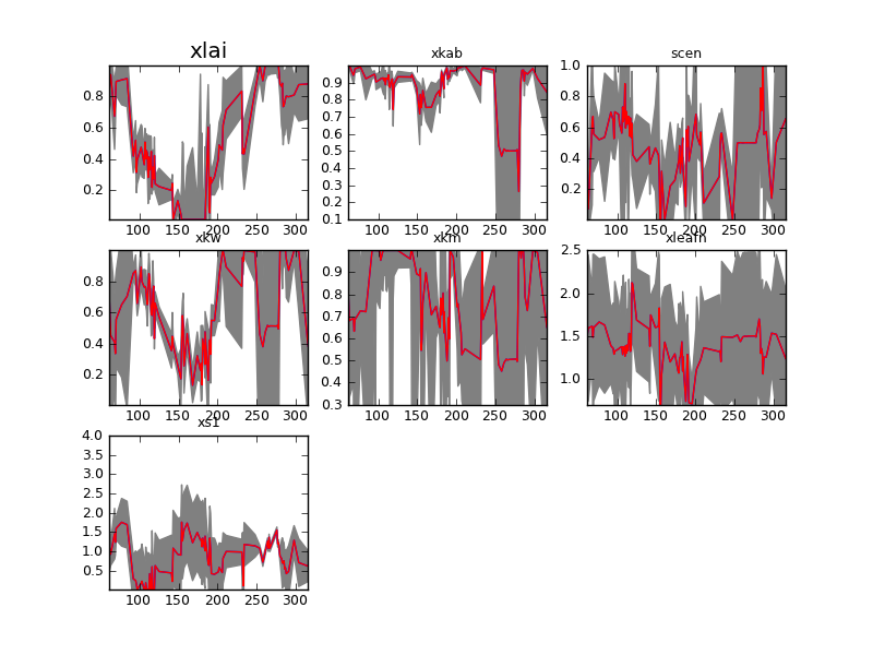
Results inverting each observation individually for a wheat field. Note that this plot is in transformed coordinates

The parameter-by-parameter smoothing using the method of Garcia (2010) results in a smoothed and complete version of the parameter evolution. We can see that this is already a fairly good estimate of the parameters. (the plot is in plots/output/brdf_WW_1_A_1.kernelFilteredSingle.dat_smooth.png)

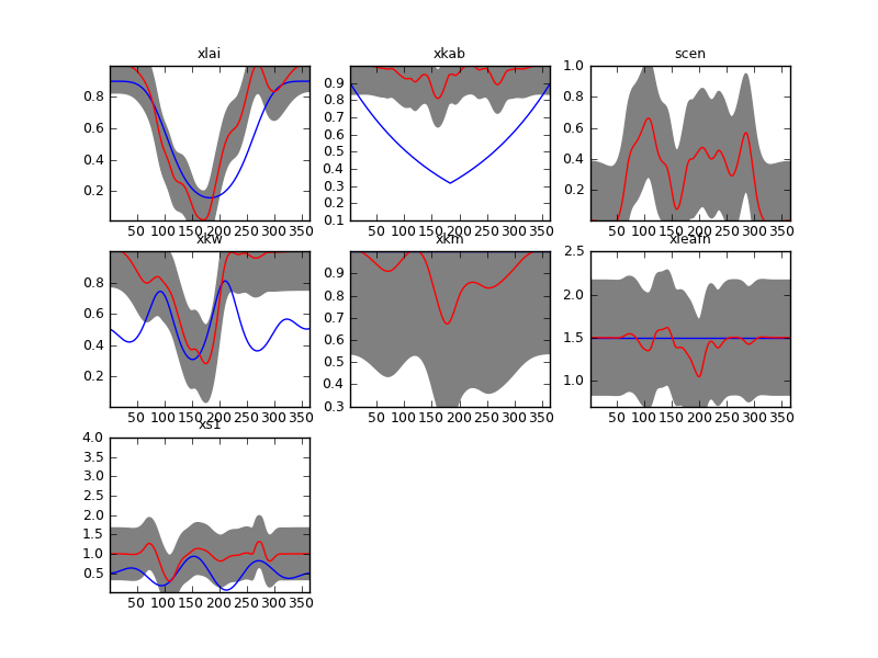
Parameter-by-parameter smoothing and interpolation. The red line shows the maximum a posteriori paremeter estimate, and the grey lines show a measure of the uncertainty. The blue line show the temporal evolution of the Sentinel synthetic experiment trajectories for comparison. Note that this plot is in transformed coordinates

Using this a starting value, we then solve the EOLDAS problem. We expect that this solution is already close the minimum, so solving the problem will be reasonably fast. We also use the \(\Gamma\) from the optimal smoothing/interpolation. While this is not exactly the same problem that we are solving in EOLDAS (different boundary conditions and limited to a second order differntial operator), we assume that there’s tolerance to \(\Gamma\) (see Lewis et al 2012). The results confirm that we only tweak the starting solution slightly: the red line (with associated grey 95% CI) is very similar in most cases to the initial value (blue line). The plot is in plots/output/brdf_WW_1_A_1.kernelFiltered.dat_Gamma00000529.png:

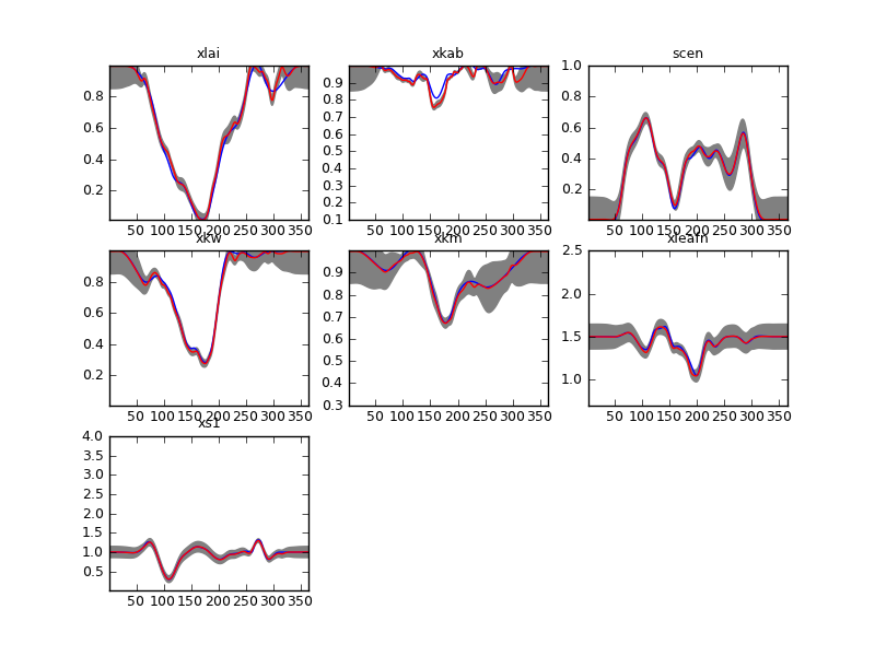
DA solution in red (plus grey 95% credible interval). The blue line shows the initial guess. Note that this plot is in transformed coordinates.

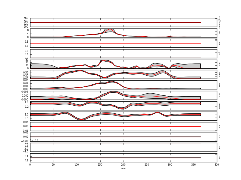
DA solution in red (plus grey 95% credible interval) in real coordinates . This plot can be found in output/brdf_WW_1_A_1.kernelFiltered.dat_result.dat.plot.x.png

The temporal evolution shown in this las plot is consistent with the development of a wheat field, and even senescence and leaf water dynamics can arguably be identified after the peak LAI period.

Some comments¶

This is nearly equivalent for solving for the dynamic model term. Since the solution is already quite close to the minimum, only slight modifications in the observation component are envisaged. Further speed-ups can be envisaged by using a linear approximation to the observation operator at this stage. Also, in a practical sense, the single inversions don’t uncertainty calculations, and a faster first pass using look-up tables might add further speed to the whole process.