Radiative transfer modelling for optical remote sensing¶

Introduction¶

Our main focus will be on using the EOLDAS data assimilation techniques to understand the land surface using optical remote sensing data. Optical sensors capture reflected solar radiation in the 400 to 2500nm range, over a number of wavebands. The signal on these bands is a combination of processes that influence the scattering of photons, such as interactions of photons within vegetation canopies, interactions with aerosols in the atmosphere, gaseous absorption processes, etc. Since all these processes contribute to the signal, it is important to have a physical understanding to separate their contributions and produce accurate estimates of the combined state of the atmosphere and land surface.

Typically, RT models of the land surface model the interactions of photons and plant components (leaves, trunks, etc.) above a surface layer (usually soil, but also snow). Atmospheric radiative transfer models are needed to account for water vapour and ozone absorption in the atmosphere, as well as for the effect of aerosols. One can think of this arrangement as a stacking of models, going from bottom to top as: soil model, vegetation model and atmospheric model.

Our main focus is the study of the land surface using DA techniques. The proposed RT models predict, for a given wavelength and acquisition geometry, directional reflectance of the land surface. The parameters that govern these models are typically to do with soil structure (soil brightness and roughness terms) and the vegetation architecture (leaf area index (LAI), leaf angle distribution, ...), as well as leaf biochemical parameters (chlorphyll a+b concentration, dry matter, leaf structural parameters...). These paraeters are the ones that form our land surface state vector, and they will vary with time and location, but provide a full description of the surface.

We note that these models are highly non-linear, and combined with only modest observations available in terms of angular and spectral sampling, as well as the contribution of thermal noise in the acquisitions, result in an*ill-posed problem*: typically, the available observations do not provide enough constrains to the models, and this results in state vector elements being poorly determined, equivalently having large uncertainties. We shall see that these situation can be improved by the use of data assimilation techniques.

We will first consider a simple RT model for continuous canopies under a soil layer, with a leaf optical model embedded. The soil layer is Lambertian, and it is assumed that its brightness at a specific waveband is a linear combination of a number of spectral basis functions. By default, these are the basis functions defined in Price 1991 , but they can be easily changed by users. Note that the model will oversimplify the directional effects of typical rough land surfaces, and that the Price spectral basis functions really only apply to soils at field capacity. Also, the effect of e.g. snow is not considered.

The leaf model is the widely used PROSPECT model, which treats leaves as a stack of thin plates. Other parameters control the absorption of energy at different wavelengths. The parameters of the PROSPECT model are

\(N\), the number of leaf layers,
\(C_{ab}\), the concentration of chlorophyll a+b \([\mu g cm^{-2}]\),
\(C_{car}\), the concentration of carotenoids \([\mu g cm^{-2}]\),
\(C_{w}\), equivalent leaf water \([cm]\),
\(C_{dm}\), dry matter \([\mu g cm^{-2}]\),
\(C_{sen}\), the proportion of senescent material (fractional, between 0 and 1).

The canopy model chosen is Semidiscrete by Gobron et al. 1997, for which an adjoint has been develoepd here to allow more rapid state estimation. This model assumes a continuous canopy and is governed by LAI, leaf area distribution (discretised into five different classes), two terms that control the so-called “hotspot” effect, and three spectral terms (one for the soil and two for leaves), which are fed in from PROSPECT and the spectral soil model. In total, the state vector has thirteen or fourteen components (four related to the soil, six or seven to the leaf properties and three to the canopy). This allows the simulation of the directional reflectance for narrow spectral wavebands and for a specified illumination/acquisition geometry.

Solving for a single observation¶

We first apply the eoldas to the problem of attempting a state estimate from a single satellite observation. These data have multiple wavebands, but we consider here only a single location and date.

An example data file for this is some MERIS data over a field site in Germany. The file is MERIS_WW_1_A_1.brf, the start of which looks like:

#BRDF 10 15 412 442 489 509 559 619 664 680 708 753 761 778 864 884 900 0.01 0.01 0.01 0.01 0.01 0.01 0.01 0.01 0.01 0.01 0.01 0.01 0.01 0.01 0.01
108 1 4.307049 286.659393 42.972881 152.909012  0.019400 0.025100 0.034100 0.035800 0.059700 0.043900 0.039200 0.039900 0.120300 0.402700 0.407500 0.417600 0.445800 0.448300 0.450100 
114 1 19.283617 288.855164 40.170044 156.520325  0.022000 0.027400 0.036100 0.038300 0.058600 0.046600 0.042400 0.043100 0.112200 0.358100 0.362600 0.372000 0.398300 0.399900 0.401000 
155 1 32.146313 291.063110 30.257147 156.645920  0.010100 0.014900 0.022500 0.027900 0.054500 0.034400 0.025000 0.024600 0.099100 0.433800 0.445200 0.469100 0.494100 0.494900 0.495500 
174 1 34.970631 291.616272 29.384569 155.618637  0.016800 0.020800 0.027200 0.031700 0.064400 0.041400 0.026400 0.024200 0.132000 0.443700 0.453600 0.474300 0.505400 0.506700 0.507600 
178 1 4.285298 286.663055 31.555040 144.463577  0.024900 0.028300 0.033600 0.037000 0.062700 0.042800 0.032500 0.031100 0.110600 0.389000 0.400600 0.424700 0.463900 0.465400 0.466500 
190 1 32.115547 291.067474 30.814306 153.679443  0.016700 0.023600 0.034600 0.042000 0.072200 0.063800 0.050200 0.047100 0.136100 0.301100 0.309100 0.325900 0.371400 0.378300 0.383500 
190 1 32.115547 291.067566 30.814367 153.679428  0.014000 0.021200 0.032700 0.040300 0.071000 0.062900 0.049300 0.046200 0.135700 0.301600 0.309700 0.326500 0.372200 0.379100 0.384300 
197 1 8.136833 287.214844 33.390018 145.816544  0.041900 0.049500 0.061600 0.069900 0.099200 0.113300 0.114200 0.115800 0.184700 0.255000 0.259600 0.269400 0.329000 0.340300 0.348800 
232 1 8.137174 287.211914 41.582573 151.810349  0.033900 0.042800 0.056700 0.062800 0.092400 0.090800 0.090300 0.092500 0.163300 0.257000 0.259700 0.265300 0.298700 0.306000 0.311400 
264 1 0.380700 206.624115 52.586159 157.652710  0.065000 0.073300 0.086500 0.089100 0.101900 0.113000 0.121000 0.124200 0.152300 0.187600 0.190100 0.195300 0.226500 0.233300 0.238400

We build a suitable configuration file config_files/meris_single.conf

# configuration file
# note that some words are protected: values, keys
# so dont use them
# other than that, you can set any level of hierarchy in the
# representation
# this next part serves no purpose other than
# to show how different options can be set

# It is a requirement that parameter.names be defined

[parameter]
location = ['time']
limits = [[1,365,1]]
names=gamma_time,xlai, xhc,  rpl,  xkab, scen, xkw, xkm,   xleafn, xs1,xs2,xs3,xs4,lad
solve = [1]*len($parameter.names)
help_solve='flags for which state vector elements to solve for'

[parameter.result]
filename = 'output/meris/MERIS_WW_1_A_1.params'
help_filename="state vector results file"
format = 'PARAMETERS'

[parameter.assoc_solve]
xkw = 0
gamma_time = 0
lad = 0
xs3 = 0
xs4 = 0
xhc = 0
rpl = 0

[parameter.x]
datatype = x
names = $parameter.names
default = [0.05]*len($parameter.names)
help_default = "Set the parameter default values"
apply_grid = True
sd = [1.]*len($parameter.names)
bounds = [[0.01,0.99]]*len($parameter.names)
####state = fullState.dat
invtransform=$parameter.names
transform=$parameter.names

[parameter.x.assoc_transform]
xlai=np.exp(-xlai/2.)
xkab=np.exp(-xkab/100.)
xkw=np.exp(-xkw*50.)
xkm=np.exp(-100.*xkm)

[parameter.x.assoc_invtransform]
xlai=-2.*np.log(xlai)
xkab=-100.*np.log(xkab)
xkw=-(1./50.)*np.log(xkw)
xkm=-(1./100.)*np.log(xkm)

[parameter.x.assoc_bounds]
gamma_time = 0.000001,100000
xlai = 0.05,0.99
xhc = 0.05,10.0
rpl = 0.01,0.10
xkab = 0.1,0.99
scen = 0.001,1.0
xkw = 0.01,0.99
xkm = 0.3,0.9
xleafn = 0.9,2.5
xs1 = 0.01, 4.
xs2 = 0.01, 5.
xs3 = 0., 0.
xs4 = 0.,0. 
lad = 1,5 


[parameter.x.assoc_default]
####gamma_time = 0.01
xlai = 0.95
xhc = 5
rpl = 0.01
xkab = 0.95
scen = 0.001
xkw = 0.95
xkm = 0.35
xleafn = 1.5
xs1 = 1.0
xs2 = 0.001
xs3 = 0
xs4 = 0
lad = 5
help_lad = 'lad value'

[general]
is_spectral = True
calc_posterior_unc=False
write_results=True
doplot=True
plotmod=20
plotmovie=True

[general.optimisation]
randomise=False

[operator]
obs.name=Observation_Operator
obs.datatypes = x,y

[operator.obs.rt_model]
model=semidiscrete1
use_median=True
help_use_median = "Flag to state whether full bandpass function should be used or not.\nIf True, then the median wavelength of the bandpass function is used"
bounds = [400,2500,1]
help_bounds = "The spectral bounds (min,max,step) for the operator'
ignore_derivative=False
help_ignore_derivative = "Set to True to override loading any defined derivative functions in the library and use numerical approximations instead"

[operator.obs.x]
names = $parameter.names[1:]
sd = [1.0]*len($operator.obs.x.names)
datatype = x

[operator.obs.y]
control = 'mask vza vaa sza saa'.split()
names = "412 442 489 509 559 619 664 680 708 753 761 778 864 884 900".split()
sd = "0.01 0.01 0.01 0.01 0.01 0.01 0.01 0.01 0.01 0.01 0.01 0.01 0.01 0.01 0.01".split()
datatype = y
state = data/meris/MERIS_WW_1_A_1.brf
help_state='set the obs state file'

[operator.obs.y.result]
filename = 'output/meris/MERIS_WW_1_A_1.fwd'
help_filename = 'forward modelling results file'
format = 'PARAMETERS'

You can note several things about the semidiscrete observation oeprator from this:

names=gamma_time,xlai, xhc,  rpl,  xkab, scen, xkw, xkm,   xleafn, xs1,xs2,xs3,xs4,lad

The (apparent) state variables, other than gamma_time that is (potentially) used for the differential operator are:

xlai : \(LAI\), the single sided leaf area per unit ground area
xhc : The canopy height
rpl : The leaf radius/dimension (same units as canopy height)
xkab : \(C_{ab}\), the concentration of chlorophyll a+b \([\mu g cm^{-2}]\),
scen : \(C_{sen}\), the proportion of senescent material (fractional, between 0 and 1).
xkw : \(C_{w}\), equivalent leaf water \([cm]\),
xkm : \(C_{dm}\), dry matter \([\mu g cm^{-2}]\),
xleafn : \(N\), the number of leaf layers,
xs1 : Soil PC1 (soil brightness)
xs2 : Soil wetness
xs3 : not used
xs4 : not used
lad : leaf angle distribution (coded 0-5). See Semidiscrete code for details.

However, the section [parameter.x.assoc_transform] contains:

####state = fullState.dat
invtransform=$parameter.names

which sets default state transformations and inverse transforms to be identity (e.g. xlai = xlai).

Then the section:

[parameter.x.assoc_transform]
xlai=np.exp(-xlai/2.)
xkab=np.exp(-xkab/100.)
xkw=np.exp(-xkw*50.)

overrides this for the specifc states mentioned to tell the eoldas that there is a transformation (in the RT model code) between true state (e.g. \(LAI\)) and the state we solve for. The reason for using a transformation is in an attempt to approximately linearise the sensitivity of \(H(x)\) to the state variable. This is a good idea generally, for avoiding getting trapped in local minima when optimising and also because Gaussian statistics are more appropriate for the linearised state. The inverse transforms are covered in the sections [parameter.x.assoc_invtransform]

[parameter.x.assoc_invtransform]
xlai=-2.*np.log(xlai)
xkab=-100.*np.log(xkab)
xkw=-(1./50.)*np.log(xkw)

The state vectors will be saved to file in their transformed form (as this is appropriate for the stored uncertainty information), but plots are generated for the inverse transformed states. The user has access to these inverse transforms in the code as x.transform and x.invtransform.

Second, we note that some of the state variables are ‘switched off’ for optimisation in the section parameter.solve. Initially, all solve states are set to 1:

solve = [1]*len($parameter.names)

Then we switch selected states to 0:

[parameter.assoc_solve]
xkw = 0
gamma_time = 0
lad = 0
xs3 = 0
xs4 = 0
xhc = 0

In the [general] section, we have set the flags:

write_results=True
doplot=True
plotmod=20

which tell eoldas to generate plots, and to keep updating them every ‘plotmod’ calls to the operator. This allows the user to visualise how the data assimilation is proceeding, by viewing the appropriate png files. The file names are formed from any results.filename fields found in a state.

Finally, we note the section [operator.obs.rt_model]. This tells the eoldas parameters specific to the operator being used. In the case of an observation operator, this must include operator.obs.rt_model.model. Here, we have:

[operator.obs.rt_model]
model=semidiscrete1
use_median=True
help_use_median = "Flag to state whether full bandpass function should be used or not.\nIf True, then the median wavelength of the bandpass function is used"
bounds = [400,2500,1]
help_bounds = "The spectral bounds (min,max,step) for the operator'
ignore_derivative=False

where we set the model to semidiscrete1, which will have been installed with the eoldas package (it is a dependency)

We can run this configuration with:

~/.local/bin/eoldas_run.py --conf=config_files/eoldas_config.conf \
  --conf=config_files/meris_single.conf \
  --parameter.limits='[[232,232,1]]' --calc_posterior_unc

which tells eoldas to solve for 8 state varibles: xlai, xkab, scen, xkw, xkm, xleafn, xs1, xs2 from any meris data found on day 232.

Here, since we are using an observation on a single data, we do not include the dynamic model, and merely attempt to solve with the observation operator. This process, with a single operator (the radiative transfer model), can also be called ‘model inversion’ where we attempt to estimate the state vector elements known (and expressed in the radiative transfer model) to control the spectral bidirectional reflectance of vegetation canopies). In truth we cannot claim that this is the optimal solution based only on the model and observations, as we also have the implicit constraint of bounds to the state estimate. This is a form of prior information that we use to help constrain the problem. Using an Identity Operator as we have done in previous exercises is, in many ways just another way of expressing this same idea, just with a different statistical distribution. With ‘hard’ bounds to the state vector elements we are assuming a ‘flat’ probability of occurrence between those bounds. If we use an Identity Operator and describe \(y\) as a Gaussian distribution, we have a ‘soft’ bound to the problem. In many cases there are physical limits to states, for example, xlai must lie in the bound [0,1] or more practically away from the edges of those bounds, (0,1). Similarly, plant height cannot physically be negative.

Results are written to output/meris/MERIS_WW_1_A_1.params:

#PARAMETERS time gamma_time xlai xhc rpl xkab scen xkw xkm xleafn xs1 xs2 xs3 xs4 lad sd-gamma_time sd-xlai sd-xhc sd-rpl sd-xkab sd-scen sd-xkw sd-xkm sd-xleafn sd-xs1 sd-xs2 sd-xs3 sd-xs4 sd-lad
 232.000000    0.050000    0.721891    5.000000    0.010000    0.780271    0.001000    0.950000    0.483895    1.752922    1.782001    1.387375    0.000000    0.000000    5.000000    0.000000    0.044455    0.000000    0.000000    0.038051    0.058349    0.000000    0.037975    0.282781    0.496276    1.024180    0.000000    0.000000    0.000000

with the foward modelled results in output/meris/MERIS_WW_1_A_1.fwd:

#PARAMETERS time mask vza vaa sza saa 412 442 489 509 559 619 664 680 708 753 761 778 864 884 900 sd-412 sd-442 sd-489 sd-509 sd-559 sd-619 sd-664 sd-680 sd-708 sd-753 sd-761 sd-778 sd-864 sd-884 sd-900
 232.000000    1.000000    8.137174  287.211914   41.582573  151.810349    0.041480    0.045971    0.057108    0.076985    0.096946    0.084620    0.082238    0.085325    0.156803    0.246357    0.251248    0.260606    0.301315    0.310495    0.317992    0.004038    0.002718    0.002205    0.003614    0.006606    0.003542    0.003993    0.006083    0.007471    0.009600    0.008233    0.009100    0.009550    0.009025    0.008834

and the original data in output/meris/MERIS_WW_1_A_1.fwd_orig:

#PARAMETERS time mask vza vaa sza saa 412 442 489 509 559 619 664 680 708 753 761 778 864 884 900 sd-412 sd-442 sd-489 sd-509 sd-559 sd-619 sd-664 sd-680 sd-708 sd-753 sd-761 sd-778 sd-864 sd-884 sd-900
 232.000000    1.000000    8.137174  287.211914   41.582573  151.810349    0.033900    0.042800    0.056700    0.062800    0.092400    0.090800    0.090300    0.092500    0.163300    0.257000    0.259700    0.265300    0.298700    0.306000    0.311400    0.010000    0.010000    0.010000    0.010000    0.010000    0.010000    0.010000    0.010000    0.010000    0.010000    0.010000    0.010000    0.010000    0.010000    0.010000

with graphics:

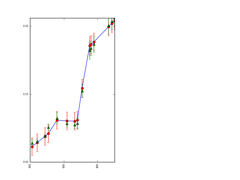
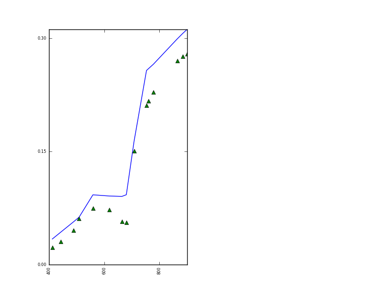
which is a plot of MERIS reflectance as a function of wavelength. The red dots show the orginal data points with assumed uncertainty shown as 95% confidence intervals (0.01 * 1.96 here). The green line is the modelled version, with the error bars indicating the 95% confidence intervals for each waveband (slightly, but not greatly lower than the prior uncertainties).

This shows that the eoldas is able to replicate the observed reflectance very well. If we can do this, then why do we need data assimilation? The answer to that comes from looking back at the solved state information.

For xlai (i.e. \(\exp(-LAI/2)\)) we retrieve a value of 0.721891, i.e. LAI of 0.652. This might well be plausible for the particular location, but we see that we have an uncertainty of 0.654474 on this. Since xlai is bounded [0,1] this means that this is a very unreliable estimate.

For some of the model states that we requested to be solved we do even worse, xkw (also bounded [0,1]) has an apparent uncertainty of 46.326810, though the reason for this is simply that the MERIS instrument does not sample at wavelengths at which reflectance is very sensitive to leaf water content. Interestingly, one of the lower uncertainties is 0.166161 for xkab. This is because MERIS does sample at several wavebands that are sensitive to chlorophyll content. The retrieved value here is 0.780574 which corresponds to a concentration of 24.8 \([\mu g cm^{-2}]\).

So, not only is our knowledge of these state variables we require actually quite poor from a single observation, but also, if we were to look at the full inverse Hessian, we would see high degrees of correlation between the state estimates.

This is not surprising: we are trying here to retrieve 8 states from measurements in 15 wavebands. We have assumed here an uncertainty of 0.01 in the surface reflectance, which could be a little high for some bands, but note that we have assumed the error independent for each wavelength, which it most certainly would not be (in that case, and in the absence of any further information on the error correlation structure, it may be appropriate to inflate the standard deviation).

On the positive side, the optimisation did at least converge to a viable solution, and gives a final value of \(J\) of around 3.83. Remember that \(J\) is essentially half the sum of the squared differences between modelled and measured reflectance, over 15 wavebands here, gives an MSE equivalent of 0.51 and a RMSE of 0.71, which we can loosely interpret as meaning that the ‘average’ departure between what we measure and what we simulate is around 0.71 standard deviations.

Simulating surface reflectance with the EOLDAS model operator¶

Even though the state estimate is a little poor, we can take it and simulate what we would see with other sensors (i.e. simulate different sensors). This demonstrates how the state vector, phrased as biophysical variables, allows us to translate information from one sensor to another (and thus allows us to combine information from multiple sensors as we shall see).

We build a configuration file for the MODIS instrument as config_files/modis_single.conf.

This is mainly the same as the meris configuration file other that a few items refering to the input state (which is the output of the meris run here: output/meris/MERIS_WW_1_A_1.params), the band names and uncertainty, and the input observations file, data/brdf_WW_1_A_1.kernelFiltered.dat.

# configuration file
# a minimal configuration file 
# with overrides for meris_single.conf

[parameter.result]
filename = 'output/modis/MODIS_WW_1_A_1.params'

[parameter.x]
state = 'output/meris/MERIS_WW_1_A_1.params'

[operator.obs.y]
names = "465.6 553.6 645.5 856.5 1241.6 1629.1 2114.1".split()
sd = "0.003 0.004 0.004 0.015 0.013 0.01 0.006".split()
state = data/brdf_WW_1_A_1.kernelFiltered.dat

[operator.obs.y.result]
filename = 'output/modis/MODIS_WW_1_A_1.fwd'

We can, for instance then run this with:

eoldas_run.py --conf=config_files/eoldas_config.conf \
    --conf=config_files/meris_single.conf \
    --parameter.limits='[[232,232,1]]' \
    --passer --conf=config_files/modis_single.conf

We need to load the MERIS configuration file before the MODIS one so that the latter overrides and options in the former. There are some dangers to using a whole string of configuration files as it can be difficult to keep track of information, but the software allows you to define as many as you want (up to any system limits to command lines etc.).

You can confirm that the configuration file loading is as you would expect by looking at the log file logs/modis_single.log. You really should look at that the first time you generate a new configuration file or you might end up mis-interpreting results.

Alternative to writing a new configuration file, we could have overridden the meris configuration settings with command line options. That has some of the same issues as having too many configuration files though as it could become difficult to keep track of information.

The flag --passer here tells eoldas not to perform parameter estimation, but just to do a ‘forward’ simulation from the state that we load.

The result we are interested in is written to output/modis/MODIS_WW_1_A_1.fwd and output/modis/MODIS_WW_1_A_1.fwd_orig:

#PARAMETERS time mask vza vaa sza saa 465.6 553.6 645.5 856.5 1241.6 1629.1 2114.1 sd-465.6 sd-553.6 sd-645.5 sd-856.5 sd-1241.6 sd-1629.1 sd-2114.1
 232.000000    1.000000   39.080000 -242.100000   38.990000    0.000000    0.050558    0.101616    0.080242    0.311520    0.450761    0.442036    0.297279    0.000000    0.000000    0.000000    0.000000    0.000000    0.000000    0.000000
 232.000000    1.000000   42.220000   51.240000   42.340000    0.000000    0.046082    0.094160    0.076048    0.295769    0.435960    0.429228    0.289747    0.000000    0.000000    0.000000    0.000000    0.000000    0.000000    0.000000

#PARAMETERS time mask vza vaa sza saa 465.6 553.6 645.5 856.5 1241.6 1629.1 2114.1 sd-465.6 sd-553.6 sd-645.5 sd-856.5 sd-1241.6 sd-1629.1 sd-2114.1
 232.000000    1.000000   39.080000 -242.100000   38.990000    0.000000    0.030300    0.054200    0.061300    0.164000    0.236200    0.224200    0.130800    0.003000    0.004000    0.004000    0.015000    0.013000    0.010000    0.006000
 232.000000    1.000000   42.220000   51.240000   42.340000    0.000000    0.053800    0.099900    0.103100    0.303700    0.319300    0.310800    0.204300    0.003000    0.004000    0.004000    0.015000    0.013000    0.010000    0.006000

with the plot in

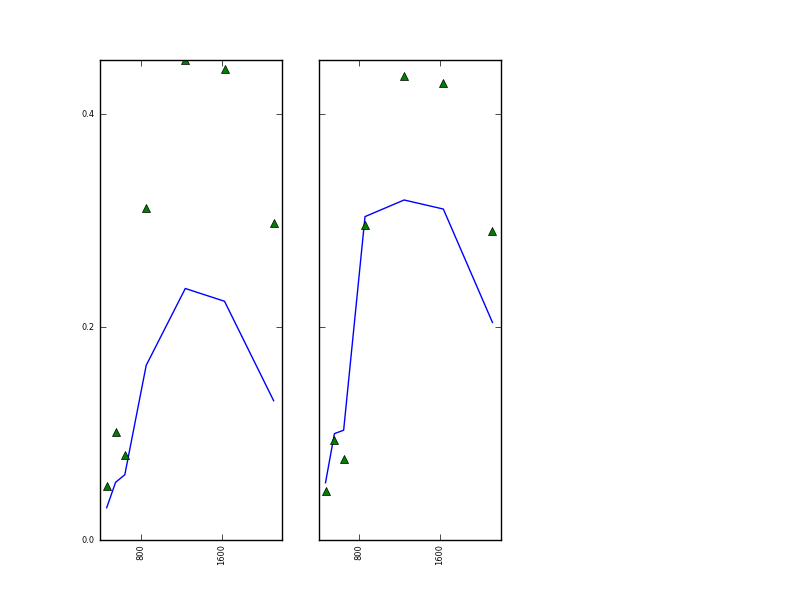
The result is rather poor for both of the MODIS observations on day 232, especially at longer wavelengths. This could be due to factors such as poor atmospheric modelling of either the MODIS or MERIS datasets, but it could equally be just due to the large uncertainty in the state estimates obtained from the MERIS data alone.

So, the information content of the MERIS data alone for a single observation only poorly constrain the estimate of the state variables. If we had some prior expactation of those states, we could use that to help constrain the estimate and we will proceed onto that in the next section.

In the meantime, it is instructive to see how we can use both the MERIS and MODIS observations to constrain the state estimate for this single day dataset.

Before that, to get an estimate from MODIS alone we create a modified form of config_files/modis_single.conf, config_files/modis_single_a.conf:

# configuration file
# a minimal configuration file 
# with overrides for meris_single.conf

[parameter.result]
filename = 'output/modis/MODIS_WW_1_A_1.params_a'

[operator.obs.y]
names = "465.6 553.6 645.5 856.5 1241.6 1629.1 2114.1".split()
sd = "0.003 0.004 0.004 0.015 0.013 0.01 0.006".split()
state = data/brdf_WW_1_A_1.kernelFiltered.dat

[operator.obs.y.result]
filename = 'output/modis/MODIS_WW_1_A_1.fwd_a'

We have changed the output filenames so as not to overwrite the previous results and remove the state definition for parameter.x (i.e. we don’t use the information from MERIS in this example).

Similarly to before, we run:

eoldas_run.py --conf=config_files/eoldas_config.conf \
  --conf=config_files/meris_single.conf --passer \
  --parameter.limits='[[232,232,1]]'  \
  --conf=config_files/modis_single_a.conf

The state estimate result is in output/modis/MODIS_WW_1_A_1.params_a

#PARAMETERS time gamma_time xlai xhc rpl xkab scen xkw xkm xleafn xs1 xs2 xs3 xs4 lad sd-gamma_time sd-xlai sd-xhc sd-rpl sd-xkab sd-scen sd-xkw sd-xkm sd-xleafn sd-xs1 sd-xs2 sd-xs3 sd-xs4 sd-lad
 232.000000    0.050000    0.950000    5.000000    0.010000    0.950000    0.001000    0.950000    0.350000    1.500000    1.000000    0.001000    0.000000    0.000000    5.000000    1.000000    1.000000    1.000000    1.000000    1.000000    1.000000    1.000000    1.000000    1.000000    1.000000    1.000000    1.000000    1.000000    1.000000

with the graphic in

This result is not particularly good, and if we examine the s of the optimisation we will see a warning: ABNORMAL_TERMINATION_IN_LNSRCH. This is simly not a viable result, even though we have wider spectral sampling than for MERIS. That may be partly down to particular characteristoics of these samples, or it might be for example that there just isn’t enough information to solve the problem (8 parameters from 7 wavebands, remember).

If we suspected it was just that the solution was trapped in some local minimum because of an inappropriate starting point for the optimisation, we could include e.g. the lines:

[parameter.result]
filename = 'output/modis/MODIS_WW_1_A_1.params_a'

in the configuration file, as the optimisation would then start from the state found from the MERIS data, but in this case that is of little value.

So, we can ‘fit’ to the MERIS data for a single date very well, but the resultant state estimates have very high uncertainty, for some state elements simply because of poor spectral sampling. And we have some MODIS data with wider spectral sampling (though fewer wavebands) but we cannot make direct use of it, even with two observations on a single day.

The obvious thing to try then is to combine the observational datasets, and this is something we can do very easily in eoldas. Even though the spectral sampling of the data is very different, we can just define different observation operators (using the same radiative transfer model) to deal with this. Of course, there are other issues to consider, such as spatial sampling/location, but the same principle applies there in a general DA system.

We can base the new configuration on that we used for MERIS, and simply declare the MODIS operator with a different name: (confs/modis_single_b.conf)

# configuration file
# a minimal configuration file 
# with overrides for meris_single.conf

[parameter.result]
filename = 'output/modis/MODIS_MODIS_WW_1_A_1.params_b'

# A New Operator
[operator]
obs_modis.name=Observation_Operator
obs_modis.datatypes = x,y

# NB -- give a new name to the meris operator output
[operator.obs.y.result]
filename = 'output/meris/MERIS_WW_1_A_1.fwd_b'

[operator.obs_modis.rt_model]
model=semidiscrete2
use_median=True
help_use_median = "Flag to state whether full bandpass function should be used or not.\nIf True, then the median wavelength of the bandpass function is used"
bounds = [400,2500,1]
help_bounds = "The spectral bounds (min,max,step) for the operator'
ignore_derivative=False
help_ignore_derivative = "Set to True to override loading any defined derivative functions in the library and use numerical approximations instead"

[operator.obs_modis.x]
names = $parameter.names[1:]
sd = [1.0]*len($operator.obs_modis.x.names)
datatype = x

[operator.obs_modis.y]
control = 'mask vza vaa sza saa'.split()
names = "465.6 553.6 645.5 856.5 1241.6 1629.1 2114.1".split()
sd = "0.003 0.004 0.004 0.015 0.013 0.01 0.006".split()
state = data/brdf_WW_1_A_1.kernelFiltered.dat
help_state='set the obs_modis state file'

[operator.obs_modis.y.result]
filename = 'output/modis/MODIS_WW_1_A_1.fwd_b'

We can then run with both meris and modis data:

eoldas_run.py --conf=config_files/eoldas_config.conf \
  --conf=config_files/meris_single.conf \
  --parameter.limits='[[232,232,1]]' \
  --conf=config_files/modis_single_b.conf

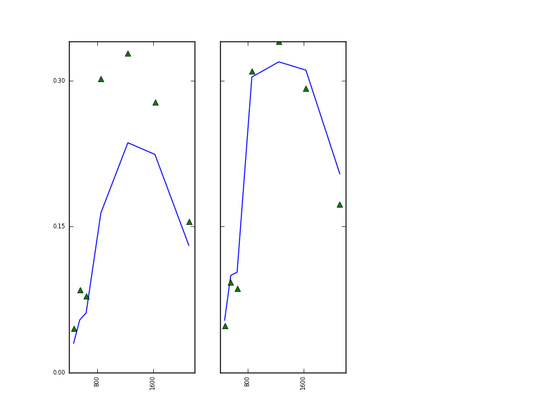
In any case, the result still does not have a good convergence, so the combination has not been a complete success.

The new (combined) state estimate is in output/modis/MODIS_MODIS_WW_1_A_1.params_b:

#PARAMETERS time gamma_time xlai xhc rpl xkab scen xkw xkm xleafn xs1 xs2 xs3 xs4 lad sd-gamma_time sd-xlai sd-xhc sd-rpl sd-xkab sd-scen sd-xkw sd-xkm sd-xleafn sd-xs1 sd-xs2 sd-xs3 sd-xs4 sd-lad
 232.000000    0.050000    0.295873    5.000000    0.010000    0.961493    0.484655    0.950000    0.650907    0.900000    0.010000    0.165705    0.000000    0.000000    5.000000    1.000000    1.000000    1.000000    1.000000    1.000000    1.000000    1.000000    1.000000    1.000000    1.000000    1.000000    1.000000    1.000000    1.000000

The new xlai value is 0.435037 with a standard deviation of 0.000730. This corresponds to a LAI of 1.66 (confidence interval 1.58 to 1.66). The xkab value though is 0.958366 which is very low (4.25) when inverse transformed. The apparent uncertainty for this (sd) is 0.018995 on xlai, so the xlai confidence interval is 0.0 to 6.25, since it is bounded at 0. These posterior estimates are probably unreliable: we can suggest that because the optimisation routine reported that it did not find a very well converged solution.

Other forms of constraint¶

We have seen that we can apply eoldas to state vector estimation using the semidiscrete canopy reflectance model. This is very much what we want to be able to do from EO data: infer characteristics of the land surface, so that is positive. However, observations from a single sensor very often have insufficient information content to reliably allow an estimate of the range of state variables we know to affect the signal. The only constraint we have applied here beyond the observations (and the model) is that of physical bounds to some of the states (N.B. in eoldas, if you want to set only an upper or lower bound, you can use None to indicate that no bound should be set).

Even though we managed a ‘stable’ retrieval from MERIS data, the resultant uncertainties were very high, which makes the value of the retrieval rather low for any practical purposes. We saw that in this case, we could not find a viable solution for the 2 MODIS samples we used. Also, we demonstrated how to use the observation operator can be used to map from one EO measurement set (the 15 MERIS wavebands) to anoth (MODIS). The comparison was poor however because of the poorly constrained estimate of the states from the MERIS data.

How then can we improve the situation? The only real answers are: (i) get sensor data with higher information content (there are practical, physical and financial limitations to that however); (ii) add other sources of information. In generating global satellite products, for example, it is common practice to assume that some of the state variables (e.g. those affecting leaf and soil reflectance) are known. This is rather a dangerous assumption and it would be better to at least phrase this supposed insight into some distribution (applying hard physical bounds which we can implement in eoldas by changing the limits of validity of the states; or assuming some statistical distribution`)

To demonstrate this, we build a new configuration file, config_files/modis_single_c.conf:

# configuration file
# a minimal configuration file 
# with overrides for meris_single.conf

[parameter.result]
filename = 'output/modis/MODIS_MODIS_WW_1_A_1.params_c'

# A New Operator
[operator]
obs_modis.name=Observation_Operator
obs_modis.datatypes = x,y
prior.name=Operator
prior.datatypes = x,y

[operator.prior.result]
filename = output/modis/MODIS_MODIS_WW_1_A_1_prior_c.dat

[operator.prior.x]
names = $parameter.names[1:]
sd = [1.0]*len($operator.prior.x.names)
datatype = x

[operator.prior.y]
names = $parameter.names[1:]
sd = 0.5,0.5,0.5,0.5,0.5,0.5,0.5,0.5,0.5,0.5,0.5,0.5,0.5
state = 0.5,5,0.01,0.5,0.5,0.5,0.5,1.5,1.0,0.0,0,0,5
datatype = x

# NB -- give a new name to the meris operator output
[operator.obs.y.result]
filename = 'output/meris/MERIS_WW_1_A_1.fwd_c'

[operator.obs_modis.rt_model]
model=semidiscrete2
use_median=True
help_use_median = "Flag to state whether full bandpass function should be used or not.\nIf True, then the median wavelength of the bandpass function is used"
bounds = [400,2500,1]
help_bounds = "The spectral bounds (min,max,step) for the operator'
ignore_derivative=False
help_ignore_derivative = "Set to True to override loading any defined derivative functions in the library and use numerical approximations instead"

[operator.obs_modis.x]
names = $parameter.names[1:]
sd = [1.0]*len($operator.obs_modis.x.names)
datatype = x

[operator.obs_modis.y]
control = 'mask vza vaa sza saa'.split()
names = "465.6 553.6 645.5 856.5 1241.6 1629.1 2114.1".split()
sd = "0.003 0.004 0.004 0.015 0.013 0.01 0.006".split()
state = data/brdf_WW_1_A_1.kernelFiltered.dat
help_state='set the obs_modis state file'

[operator.obs_modis.y.result]
filename = 'output/modis/MODIS_WW_1_A_1.fwd_c'

The only new sections are:

[operator]
obs_modis.name=Observation_Operator
obs_modis.datatypes = x,y
prior.name=Operator
prior.datatypes = x,y

[operator.prior.result]
filename = output/modis/MODIS_MODIS_WW_1_A_1_prior_c.dat

[operator.prior.x]
names = $parameter.names[1:]
sd = [1.0]*len($operator.prior.x.names)
datatype = x

[operator.prior.y]
names = $parameter.names[1:]
sd = 0.5,0.5,0.5,0.5,0.5,0.5,0.5,0.5,0.5,0.5,0.5,0.5,0.5
state = 0.5,5,0.01,0.5,0.5,0.5,0.5,1.5,1.0,0.0,0,0,5
datatype = x

which state that the operator (called operator.prior) is to have \(H(x) = I(x)\) (we call the operator Operator, the default) and we, simplistically here, set the state and standard deviation to 0.5. This then is a quite loose constraint as most states are bounded [0,1].

We run now with:

eoldas_run.py --conf=config_files/eoldas_config.conf \
  --conf=config_files/meris_single.conf \
  --parameter.limits='[[232,232,1]]' \
  --conf=config_files/modis_single_c.conf

Now, we get convergence, with the results in output/modis/MODIS_WW_1_A_1.params_c:

#PARAMETERS time gamma_time xlai xhc rpl xkab scen xkw xkm xleafn xs1 xs2 xs3 xs4 lad sd-gamma_time sd-xlai sd-xhc sd-rpl sd-xkab sd-scen sd-xkw sd-xkm sd-xleafn sd-xs1 sd-xs2 sd-xs3 sd-xs4 sd-lad
 232.000000    0.050000    0.295724    5.000000    0.010000    0.961483    0.484544    0.950000    0.651112    0.900000    0.010000    0.157713    0.000000    0.000000    5.000000    1.000000    1.000000    1.000000    1.000000    1.000000    1.000000    1.000000    1.000000    1.000000    1.000000    1.000000    1.000000    1.000000    1.000000

One particular thing to note here is that all of the uncertainties are now less that 0.5. This happens (simply?) because: we set the prior uncertainty to 0.5.

Note

Think about why that happens, statistically... essentially because \(C_{post}^{-1} = C_{a}^{-1} + C_{prior}^{-1}\).

That is fine, and, as we have noted, expected (indeed we can think of that being the main purpose of applying the prior constraint), but it does mean that users of eoldas must bear in mind the consequences of setting too tight constraints as they will result in apparently low posterior uncertainties.

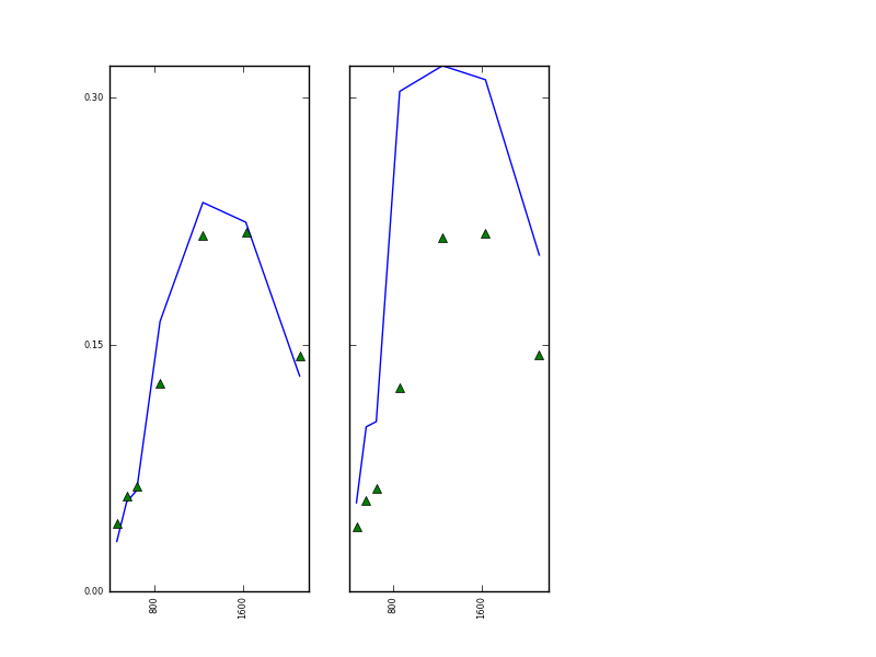
The original and forward modelled MODIS data resulting from this are:

and the MERIS:

The reproduction of the observations is clearly not wonderful, indicating some other issues with the data or model, but at least we have demonstrated how a prior can be used in eoldas to help condition the solution. As indicated above, one has to be careful applying prior constraints, as the results can be very dependent on the values chosen, but really such care must be taken about all choices here (which model, which data etc.).

Summary¶

In this section, we have moved from applying simple operators where the domain of the state vector and observations was the same to a more typical and useful case (for EO interpretation and use), where they are not. We have introduced a physically-based radiative transfer tool as the operator function (one that is provided with an adjoint for (relatively) rapid optimisation of the combined cost functions \(J\).

We have shown how eoldas configuration files can be progressively modified (and used in combination) to set up particular problems. We have obttained an estimate of biophysical parameters from MODIS data (failed to converge for observations on a single date), from MERIS data, and from both MODIS and MERIS combined.

This is already quite a powerful tool, but we will see in the next section that other constraints can be interesting as well.