Reprojecting and resampling data

A common problem

The previous section demonstrated how to save raster data. However, in many cases, there’s a need to reproject and resample this data. A pragmtic solution would use gdalwarp and do this on the shell. On the one hand, this is convenient, but sometimes, you need to perform this task as a intermediate step, and creating and deleting files is tedious and error-prone. Ideally, you would have a python function that would perform the projection for you. GDAL allows this by defining in-memory raster files. These are normal GDAL datasets, but that don’t exist on the filesystem, only in the computer’s memory. They are a convenient “scratchpad” for quick intermediate calculations. GDAL also makes available a function, gdal.ReprojectImage that exposes most of the abilities of gdalwarp. We shall combine these two tricks to carry out the reprojection. As an example, we shall look at the case where the NDVI data for the British Isles mentioned in the previous section needs to be reprojected to the Ordnance Survey National Grid, an appropriate projection for the UK.

The main complication comes from the need of gdal.ReprojectImage to operate on GDAL datasets. In the previous section, we saved the NDVI data to a GeoTIFF file, so this gives us a starting dataset. We still need to create the output dataset. This means that we need to define the geotransform and size of the output dataset before the projection is made. This entails gathering information on the extent of the original dataset, projecting it to the destination projection, and calculating the number of pixels and geotransform parameters from there. This is a (heavily commented) function that performs just that task:

def reproject_dataset ( dataset, \
            pixel_spacing=5000., epsg_from=4326, epsg_to=27700 ):
    """
    A sample function to reproject and resample a GDAL dataset from within 
    Python. The idea here is to reproject from one system to another, as well
    as to change the pixel size. The procedure is slightly long-winded, but
    goes like this:
    
    1. Set up the two Spatial Reference systems.
    2. Open the original dataset, and get the geotransform
    3. Calculate bounds of new geotransform by projecting the UL corners 
    4. Calculate the number of pixels with the new projection & spacing
    5. Create an in-memory raster dataset
    6. Perform the projection
    """
    # Define the UK OSNG, see <http://spatialreference.org/ref/epsg/27700/>
    osng = osr.SpatialReference ()
    osng.ImportFromEPSG ( epsg_to )
    wgs84 = osr.SpatialReference ()
    wgs84.ImportFromEPSG ( epsg_from )
    tx = osr.CoordinateTransformation ( wgs84, osng )
    # Up to here, all  the projection have been defined, as well as a 
    # transformation from the from to the  to :)
    # We now open the dataset
    g = gdal.Open ( dataset )
    # Get the Geotransform vector
    geo_t = g.GetGeoTransform ()
    x_size = g.RasterXSize # Raster xsize
    y_size = g.RasterYSize # Raster ysize
    # Work out the boundaries of the new dataset in the target projection
    (ulx, uly, ulz ) = tx.TransformPoint( geo_t[0], geo_t[3])
    (lrx, lry, lrz ) = tx.TransformPoint( geo_t[0] + geo_t[1]*x_size, \
                                          geo_t[3] + geo_t[5]*y_size )
    # See how using 27700 and WGS84 introduces a z-value!
    # Now, we create an in-memory raster
    mem_drv = gdal.GetDriverByName( 'MEM' )
    # The size of the raster is given the new projection and pixel spacing
    # Using the values we calculated above. Also, setting it to store one band
    # and to use Float32 data type.
    dest = mem_drv.Create('', int((lrx - ulx)/pixel_spacing), \
            int((uly - lry)/pixel_spacing), 1, gdal.GDT_Float32)
    # Calculate the new geotransform
    new_geo = ( ulx, pixel_spacing, geo_t[2], \
                uly, geo_t[4], -pixel_spacing )
    # Set the geotransform
    dest.SetGeoTransform( new_geo )
    dest.SetProjection ( osng.ExportToWkt() )
    # Perform the projection/resampling 
    res = gdal.ReprojectImage( g, dest, \
                wgs84.ExportToWkt(), osng.ExportToWkt(), \
                gdal.GRA_Bilinear )
    return dest
    

The function returns a GDAL in-memory file object, where you can ReadAsArray etc. As it stands, reproject_dataset does not write to disk. However, we can save the in-memory raster to any format supported by GDAL very conveniently by making a copy of the dataset. This literally takes two lines of code.

We expand the main part of the program to (i) save the result of the reprojection as a GeoTIFF file, (ii) read the resulting datafile and (iii) plot it:

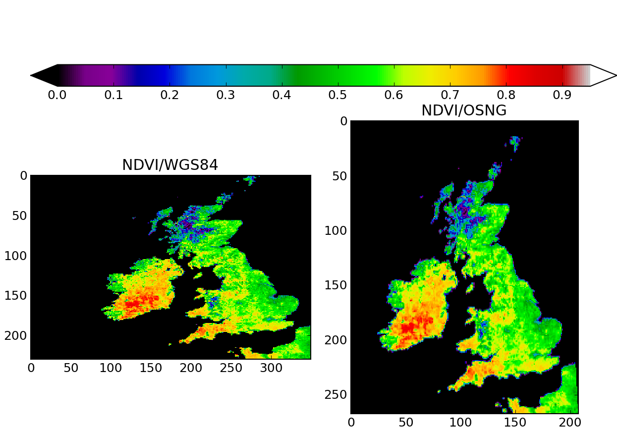
if __name__ == "__main__":
    red_filename = "red_2005001_uk.vrt"
    nir_filename = "nir_2005001_uk.vrt"
    
    ndvi = calculate_ndvi ( red_filename, nir_filename )
    save_raster ( "./ndvi.tif", ndvi, red_filename )
    # Data is now produced and saved. We can try to open the file and read it
    fig = plt.figure( figsize=(8.3,5.8 ))
    plt.subplot( 1,2,1 )
    do_plot ( "ndvi.tif", "NDVI/WGS84" )
    plt.subplot( 1,2,2 )
    # Now, reproject and resample the NDVI dataset
    reprojected_dataset = reproject_dataset ( "ndvi.tif" )
    # This is a GDAL object. We can read it
    reprojected_data = reprojected_dataset.ReadAsArray ()
    # Let's save it as a GeoTIFF.
    driver = gdal.GetDriverByName ( "GTiff" )
    dst_ds = driver.CreateCopy( "./ndvi_osng.tif", reprojected_dataset, 0 )
    dst_ds = None # Flush the dataset to disk
    # Data is now saved. We can try to open the file and read it
    do_plot ( "ndvi_osng.tif", "NDVI/OSNG" )
    cax = fig.add_axes([0.05, 0.8, 0.95, 0.05])
    cbase = matplotlib.colorbar.ColorbarBase( cax, cmap=plt.cm.spectral, \
        norm=matplotlib.colors.normalize(0,0.95), orientation='horizontal', \

The result of running the whole script is shown below

Try it out

1. Compare the produced NDVI with the official one in the HDF product (extract the area of interest to a VRT file).
2. Have a look at the QA flags (you may find this table useful). Antyhing interesting?
3. In the NDVI directory there’s NDVI data for a whole year. Can you plot an annual series of NDVI?
4. The NDVI HDF files also have a blue band, that you can use to calculate the EVI (Enhanced Vegetation Index). The formula for this is index can be found here. Repeat the above exercise with the EVI, and compare EVI and NDVI results.