Assimilating EO data into an ecosystem model with a particle filter
- The aim of today's practical is to explore the blending of observations and models
- You will use the DALEC ecosystem model, that tracks the fate of C through photosynthesis, biomass allocation and decomposition.
- We will use observations of LAI from space-borne sensors to keep the model in track
- The observations will be combined with the model using a type of particle filter (a sequential Metropolis-Hastings filter)
- We will focus on the Metolius Young Pine FLUXNET site, and will compare assimilation results to flux tower data.
The DALEC model
The DALEC model is a simple box model of C cycling.

- Carbon is acquired through the GPP box, which uses the very simple ACM model to model photosynthesis as a function of $LAI$, and temperature, incoming radiation, $CO_2$ concentration and VPD.
- Part of the GPP is lost as autototrophic respiration, to get NPP.
- The NPP is allocated to the foliar, woody and roots pools.
- The foliar and root pools loose C to the litter pool.
- The woody biomass pool looses C to the SOM/Woody debris pool.
- The litter pool decomposes into the SOM pool
- Both litter and SOM pools release C back to the atmopshere through microbial activity and heterotrophic respiration
- The DALEC model has been calibrated for the Metolius site
- We have a fairly rough understanding of the different C pools at around 2000.
- However, the DALEC model is very simplistic!!!
- The idea is that this simple model can be made to track observations, and hence combine heterogeneous observational streams into a consistent story of what's happening to C.
The MODIS observations
- We will use the MODIS LAI product, which provides both an estimate of LAI and of uncertainty in LAI.
- This product takes the red and nir reflectance, and maps them to LAI.
- The uncertainty of the LAI product is controlled by things like cloudiness, snow, etc.
In [6]:
import numpy as np
import matplotlib.pyplot as plt
%matplotlib inline
d=np.loadtxt("Metolius_MOD15_LAI.txt")
plt.figure(figsize=(10,10))
x = np.arange( 166 )
plt.plot ( x, d[:, 2], 'o' )
plt.vlines ( x, d[:, 2] - d[:, 3], d[:, 2] + d[:, 3] )
plt.xlabel("Observation time[-]")
plt.ylabel(r'LAI $m^2m^{-2}$')
Out[6]:

The particle filter
- We will use the Dowd 2007 sequential MH PF
- The model of our dynamic system is given by
- The first equation encodes the forward propagation of the state in time using the model
- The second couples the state with the observations
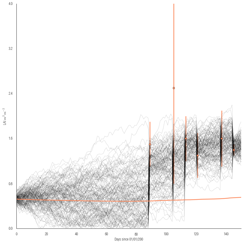
- We will couple the foliar C pool $C_f$ with observed LAI from MODIS, noting that they are related by the SLA (assumed known).
- The filter propagates a number of particles that determine the state using the model, and addss a random forcing
- If an observation is available, then particles which are able to better explain the observation (i.e., where the foliar C pool scaled by SLA is close to the observed LAI) will tend to dominate, whereas particles that are far from the LAI observation will tend to be rejected.
- After a few iterations, the trajectory ought to start tracking the observations.
In [ ]: