Inferring the characteristics of the surface from optical data

J Gómez-Dans (NCEO & UCL)

• RT theory allows us to explain the scattering & absorption of photons
• ... by describing the optical properties and structure of the scene
• However, we want to find out about the surface from the data!
• E.g. we want to infer LAI, chlorophyll, ... from reflectrance measurements
• The inverse problem....

The inverse problem

• An RT model $\mathcal{H}$ predicts directional reflectance factor, $\vec{\rho}_{m}(\Omega, \Omega')$
  • $\dots$ as a function of a set of input parameters: LAI, chlorophyll concentration, equivalent water thickness...
• $\mathcal{H}$ combination leaf RT model, canopy RT model and soil RT model
  • PROSPECT (Liberty?)
  • SAIL (ACRM, Semidiscrete, ...)
  • Linear mixture of spectra assuming Lambertian soil (Walthall, Hapke, ...)
• For this lecture, we'll refer to $\mathcal{H}$ as the observation operator
• Stack input parameters into vector $\vec{x}$.
• Other information e.g. illumination geometry, etc

$$ \mathcal{H}(\mathbf{x}, I) = \vec{\rho}_m(\Omega, \Omega') $$

• Our task is to infer $\vec{x}$ given observations $\vec{\rho}(\Omega, \Omega')$

• The model couples the observations and our parameters
• In some cases, we might be able to provide an analytic inversion
• However, we have ignored observational uncertainties
• We have also ignored the model uncertainty (inadequacy): a model is not reality
• These uncertainties will translate into uncertainty into our inference of $\vec{x}$
• Is there a framework for this?

• Least squares: minimise data-model mismatch
• Assuming observational noise,

$$ \mathcal{H}(\mathbf{x}, I) = \vec{R}_m(\Omega, \Omega') $$

• Any solution that falls within the error bars cannot be discarded

$$ \|\mathcal{H}(\vec{x}, I) - \vec{R}\|^2 \le \epsilon_{obs} $$

• Moreover, models very linear
• Haven't even considered model inadequacy!

• Eg simulate some healthy wheat canopy (LAI=4.2), and then run our RT model with random inputs
• Accept solutions that fall within the observational error... ($\Rightarrow$ brute force montecarlo!)

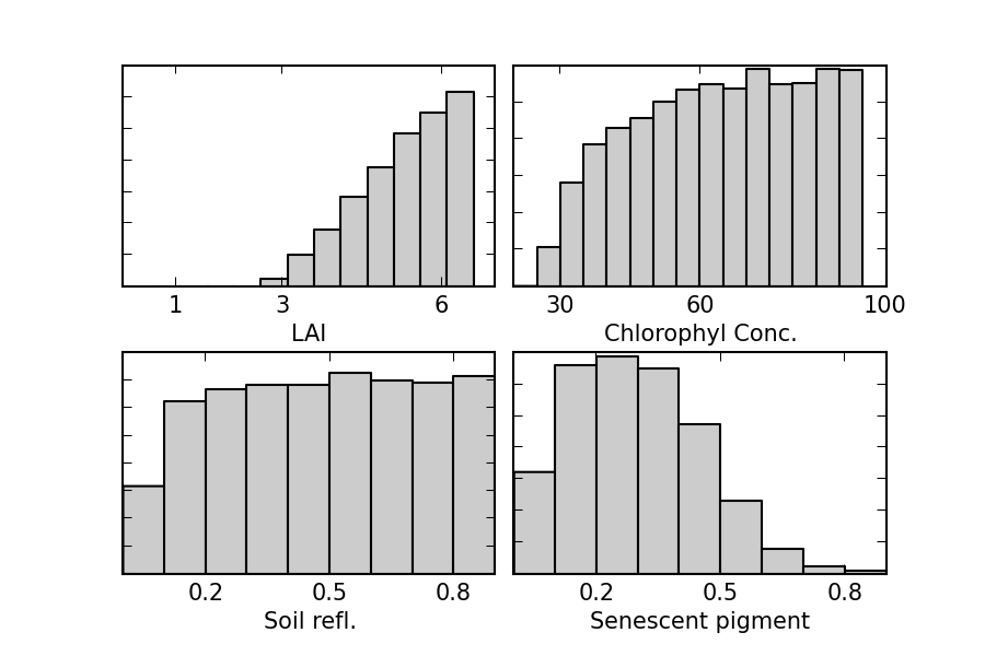
• Large uncertainty in estimate of state.
• $\Rightarrow$ limited information content in the data.
• Need more information..
  • Add more observations
  • Decrease observational uncertainty
• Need to consider sensitivity of the model.

Reverend Bayes to the rescue

• We assume that parameter uncertainty can be encoded if we treat $\vec{x}$ as a probability density function (pdf), $p(\vec{x})$.
  • $p(\vec{x})$ encodes our belief in the value of $\vec{x}$
  • Natual treatment of uncertainty
• We are interested in learning about $p(\vec{x})$ conditional on the observations $\vec{R}$, $p(\vec{x}|\vec{R})$.
• Bayes' Rule states how we can learn about $p(\vec{x}|\vec{R})$
• In essence, Bayes' rule is a statement on how to update our beliefs on $\vec{x}$ when new evidence crops up

$$ p(\vec{x} | \vec{R}, I ) =\frac{ p (\vec{R} | \vec{x}, I)\cdot p(\vec{x},I)}{p(\vec{R})}\propto p (\vec{R} | \vec{x}, I)\cdot p(\vec{x},I) $$

• $p(\vec{R}|\vec{x},I)$ is the likelihood function
  • encodes the probability of $\vec{R}$ given $\vec{x}$, and any other information ($I$)
• $p(\vec{x})$ is our a priori belief in the pdf of $\vec{x}$
• $p(\vec{R}$ can be thought of as normalisation constant, and we'll typically ignore it
• A way to picture Bayes' rule:

$$ p(\textsf{Hypothesis} | \textsf{Data},I) \propto p(\textsf{Data} | \textsf{Hypothesis},I) \times p(\textsf{Hypothesis} | I) $$

The prior $p(\vec{x})$

• Encodes everything we know about $\vec{x}$ before we even look at the data
• In some cases, we can have uninformative priors...
• ... but the real power is that it allows us to bring understanding, however weak to the problem!

The likelihood $p(\vec{R}|\vec{x})$

• The likelihood states is our data generative model
• It links the experimental results with the quantity of inference
• It includes our observations, their uncertainties, but also the model and its uncertainties

• Assume that our model is able perfect (ahem!), so if $\vec{x}$ is the true state, the model will predict the observation exactly
• Any disagreement has to be due to experimental error. We'll assume it's additive:

$$ \vec{R}=\mathcal{H}(\vec{x}) + \epsilon $$

• Assume that $\epsilon \sim \mathcal{N}(\vec{\mu},\mathbf{\Sigma}_{obs})$
  • For simplicity, $\vec{\mu}=\vec{0}$

• The likelihood is then given by $$ p(\vec{R}|\vec{x})\propto\exp\left[-\frac{1}{2}\left(\vec{R}-\mathcal{H}(\vec{x})\right)^{\top}\mathbf{\Sigma}_{obs}^{-1}\left(\vec{R}-\mathcal{H}(\vec{x})\right)\right] $$

• Have you ever seen this function?

  • Maybe its univariate cousin...
• Can you say something about (i) the shape of the function and (ii) interesting points?

The posterior

• We can simply multiply the likelihood and prior to obtain the posterior
  • In most practical applications with a non-linear $\mathcal{H}$, there is no closed solution
  • However, if $\mathcal{H}$ is linear ($\mathbf{H}$), we can solve directly
• Simple 1D case, assuming Gaussian likelihood & prior:
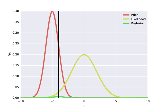
• What can you say about the information content of the data in this synthetic example?

Some simple 1D Gaussian maths...

• Try to infer $x$ from $y$, using an identity observation operator (i.e., $x=y$, so $\mathcal(x)=1$ and Gaussian noise:

$$ p(y|x) = \frac{1}{\sqrt{2\pi}\sigma_{obs}}\exp\left[-\frac{1}{2}\frac{(x-y)^2}{\sigma_{obs}^2}\right]. \qquad\text{Likelihood} $$

• Assume that we only know that $x$ is Gaussian distributed with $\mu_p$ and $\sigma_0$:

$$ p(x) = \frac{1}{\sqrt{2\pi}\sigma_0}\exp\left[-\frac{1}{2}\frac{(x-\mu_p)^2}{\sigma_0^2}\right]\qquad\text{Prior} $$$$ p(x|y) \propto \frac{1}{\sigma_{obs}\sigma_0}\exp\left[-\frac{1}{2}\frac{(x-\mu_p)^2}{\sigma_0^2}\right]\cdot \exp\left[-\frac{1}{2}\frac{(x-y)^2}{\sigma_{obs}^2}\right].\qquad\text{Posterior} $$

• The posterior distribution is indeed a Gaussian, and its mean and std dev can be expressed as an update on the prior values
  • Weighted by the relative weighting of the uncertainties

$$ \mu_p = \mu_0 + \frac{\sigma_0^2}{\sigma_0^2 + \sigma_{obs}^2}(y - \mu_0). $$$$ \sigma_p^2 = \sigma_0^2\cdot \left( 1- \frac{\sigma_0^2}{\sigma_0^2 + \sigma_{obs}^2} \right) $$

• If we now had a new measurement made available, we could use the posterior as the prior, and it would get updated!

Ill posed problems

• Stepping back from Bayes, consider the logarithm of the likelihood function:

$$ \log_{e}\left(p(\vec{R}|\vec{x})\right)\propto-\frac{1}{2}\left(\vec{R}-\mathcal{H}(\vec{x})\right)^{\top}\mathbf{\Sigma}_{obs}^{-1}\left(\vec{R}-\mathcal{H}(\vec{x})\right) $$

• Maximum occurs when the model matches the observatios
• So we can just maximise the model-data mismatch and be done, right?
• Remember our generative model, and think what this implies:

$$ \|\mathcal{H}(\vec{x}, I) - \vec{R}\|^2 \le \epsilon_{obs} $$

• Formally, any solution that falls within the error bars is a reasonable solution

Priors

• Simplest prior constraints might encode
  • range of parameters
  • physical limits of parameters (e.g. a mass must be $>0$)
• More sophisticated priors might encode more subtle information such as
  • expected values from an expert assessment
  • expected values from a climatology
• It is usually hard to encode the prior information as a pdf
  • We tend to use Gaussians as easy to parameterise

Variational solution

• If prior(s) & likelihood Gaussian...
• And if all terms are linear
• $\Rightarrow$ can solve for posterior by minimising $J(\vec{x})$:

$$ J(\vec{x})= \overbrace{\frac{1}{2}\left[\vec{x}-\vec{\mu_{x}}\right]^{\top}\mathbf{C}_{prior}^{-1}\left[\vec{x}-\vec{\mu_{x}}\right]}^{\textrm{Prior}} + \underbrace{\frac{1}{2}\left[\vec{R}-\mathcal{H}(\vec{x})\right]^{\top}\mathbf{C}_{obs}^{-1}\left[\vec{R}-\mathcal{H}(\vec{x})\right]}^{\textrm{Observation}} + \cdots $$

• You can add more constraints (more observations, more prior constraints...)
• Uncertainty given by inverse of Hessian @ minimum of $J(\vec{x})$
  • Matrix of second derivatives
• Also works OK for weakly non-linear systems!

More subtle priors

• What about the expectation of
  • spatial correlation of the state
  • temporal correlation of the state?
• Can encode expectation of smoothness in the prior
• What if we have a model of e.g. LAI evolution with e.g. thermal time?
• ... Or a full-blown vegetation/crop model?

The concept of a model

• Smoothness constraint is a simple vegetation model
  • LAI today = LAI tomorrow
• This temporal evolution model is WRONG
• More complex mode likely to also be wrong $\Rightarrow$ uncertainty!
• Encode "closeness to model" $\mathcal{M}(\vec{x})$ constraint as a Gaussian pdf: $$ p(\vec{x}|\mathcal{M},I_m)\propto -\frac{1}{2}\exp\left[ - (\vec{x} - \mathcal{M}(I_m)^{\top}\mathbf{C}_{model}^{-1}(\vec{x} - \mathcal{M}(I_m)\right] $$

Simplest model

• Smoothness $$ x_{k+1} = x_{k} + \mathcal{N}(0,\sigma_{model}) $$

• We can encode this as a matrix, if e.g. we stack $x$ over time in a vector...: $$ \begin{pmatrix} 1 &-1& 0 & 0 & \cdots\\ 0 &1 &-1 & 0 & \cdots \\ \vdots & \vdots & \vdots & \vdots & \cdots \\ \end{pmatrix}\vec{x} $$

• It's a linear form!

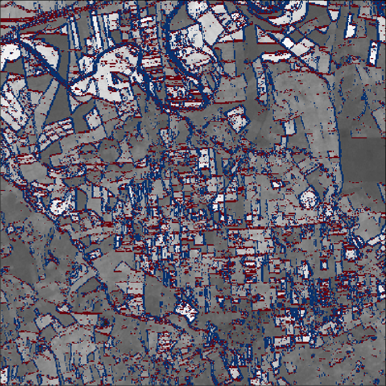
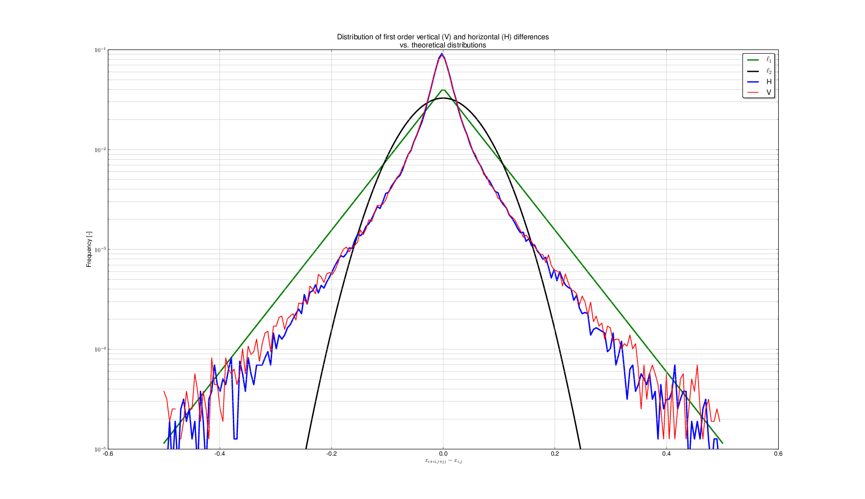
• Model can also be applied in space ($\Rightarrow$) Markov Random Field

Spatial example

• Agricultural irrigation area near Córdoba
• Landsat TM NDVI map

• Vertical (red) and horizontal (blue) differences between neighbouring pixels
• Over a given threshold

eoldas_ng

• Python tool that allows you to build variational EO problems
• In development
• Main bottleneck: slow RT models
  • Emulation of models

Final remarks

• Inversion of a model to infer input parameters is ill posed
• You need to add more information
  • priors
  • more observations
• Track all the uncertainties
• Physically consistent way of merging observations
• Variational solution can be efficient
• Apply smoothness and model constraints as priors
• eoldas_ng tool