- In the previous Session we looked at RT modelling of leaves
- Now we will consider a full canopy
- We will just the basics, as the aim is that you can start using well-established RT models
- Obviously, lots more to cover!
- We will mostly consider a turbid medium canopy
- That is a random volume of leaves and air
- In the optical domain, the size of the objects is $>>\lambda$

Define the canopy
- Vertical leaf area density function $u_{L}(z)\,\left(m^{2}m^{-3}\right)$,
- Vertical leaf number density function (e.g. the number of particles per unit volume), $N_{v}(z)\,\left(N\,particles\, m^{-3}\right)$
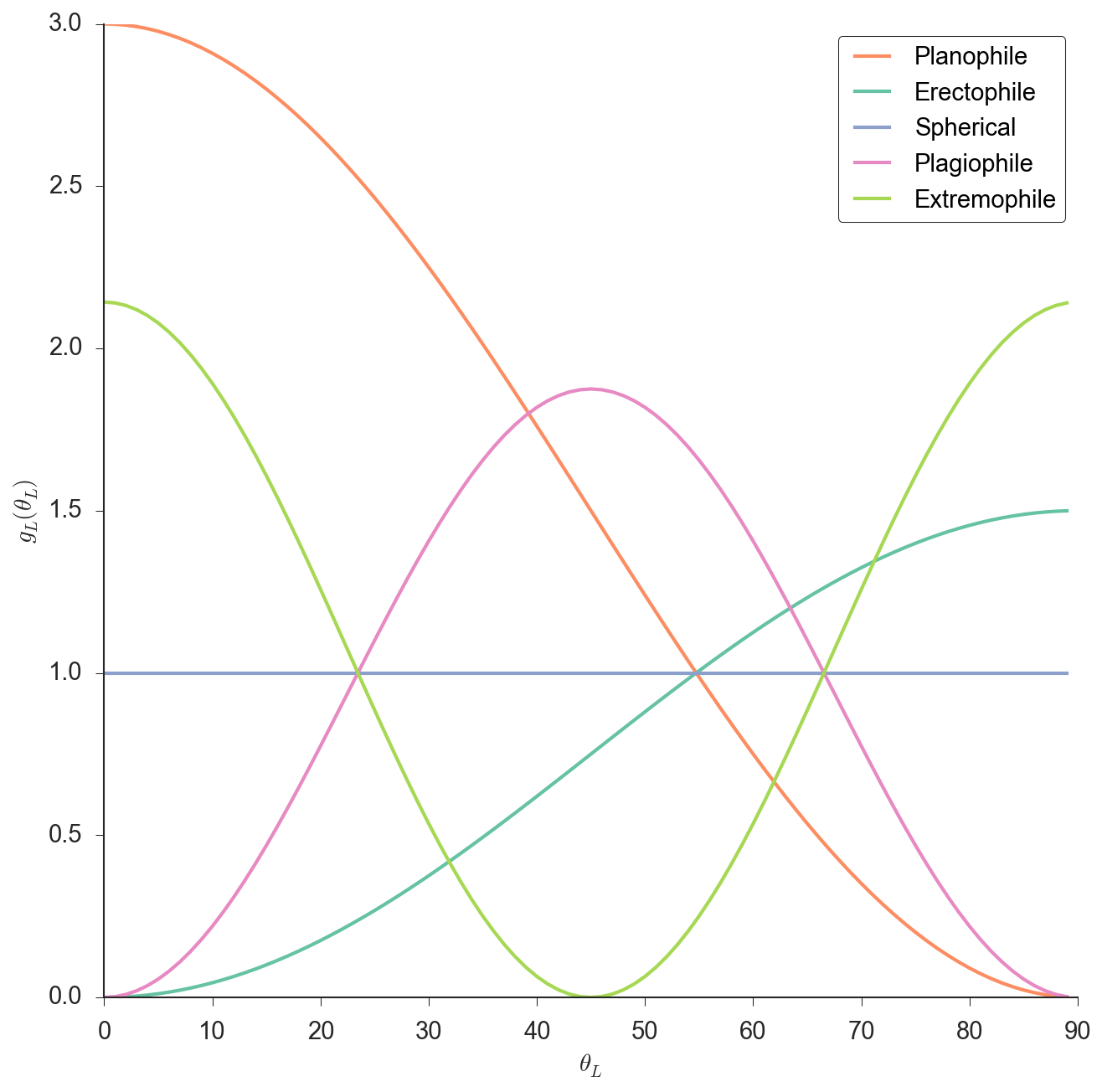
- Distribution of the leaf normal angles, $g_{L}(z, \vec{\Omega}_{L})$ (dimensionless),
- Leaf size distribution, defined as area density to leaf number density and thickness.

Some examples of leaf angle distribution functions
The radiative transfer equation
The RTE describes the change of incident radiance intensity at a specific height and direction $I(z,\vec{\Omega})$.
$$ \mu\cdot\frac{\partial I(z,\vec{\Omega})}{\partial z} = \overbrace{-\kappa_{e}\cdot I(z,\vec{\Omega})}^{\textsf{Attenuation}} + \underbrace{J_{s}(z,\vec{\Omega})}_{\textsf{Volume scattering}}, $$Attenuation
- Attenuation is governed by Beer's Law $$ I(z)=I(0)\exp(-\kappa_{e}\cdot z)=I(0)\exp(-\kappa_e\cdot LAI) $$
- $\kappa_{e}$ is the product of the medium's particle density and the extinction x-section
- Also split into radiation absorbed and scattered away in other directions.
- Remember that $LAI = \int_{z=0}^{z=-H}u_{L}(z)dz$
- Q What value of LAI is needed to intercept 99% of the radiation if $\kappa=1$?
- What if your particles (leaves) are oriented?
- We need to project the leaf area density across the beam direction $\vec{\Omega}$
- We project the leaf angle distribution function $u_{L}(z)$ using into $\vec{\Omega}$ by multiplying by
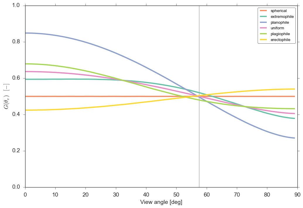
- From the previous slide, we have that
where $\kappa_{e}=G(\vec{\Omega})/\mu$.
So...
- Attenuation is a function of
- Leaf area
- leaf angle distribution
- direction of propagation
- What happens to $\kappa_e$ when...
- Sun is overhead, vertical leaves?
- Leaves are horizontal?
- Zenith angle is low?
- Zenith angle is high?
- At around $\sim 1 rad$ angle?
Volume scattering
$$ J_{s}(z,\vec{\Omega}) = \int_{4\pi} P(z,\vec{\Omega}'\rightarrow\vec{\Omega})\cdot I(\vec{\Omega}',\vec{\Omega})d\vec{\Omega}' , $$- Indicates scattered incoming radiation from all directions into the viewing direction $\vec{\Omega}$.
- $P(\cdot)$ is the phase function
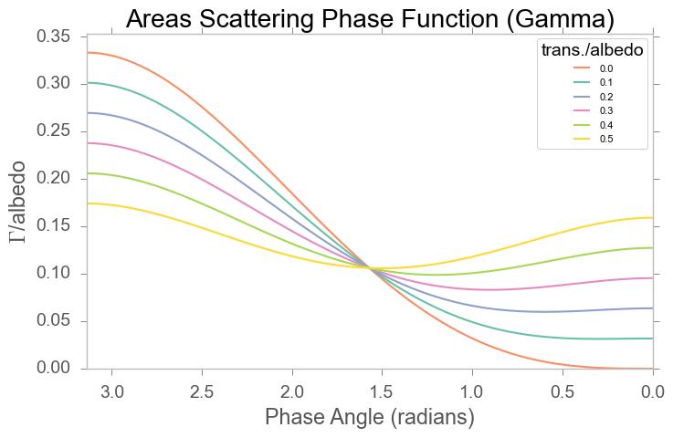
- In the optical domain, we tend to specify $P(\cdot)$ as a function of leaf area density and an area scattering function $\Gamma(\cdot)$.
- $\Gamma$ is a double projection of the leaf angle distribution, modulated by the directional reflectance (upper hemisphere) and transmittance (lower hemisphere)
- This is quite similar to $G$
Typically, we assume leaves to be bi-Lambertian, so simplify.... $$ \Gamma\left(\vec{\Omega}'\rightarrow\vec{\Omega}\right) = \rho_{L}\cdot\Gamma^{\uparrow}(\vec{\Omega}, \vec{\Omega}') + \tau_{L}\cdot\Gamma^{\downarrow}(\vec{\Omega}, \vec{\Omega}') $$
Also, if we assume $\rho\sim\tau$ (or a linear function), $\Gamma$ is a weighting of the upper and lower double projections of the leaf angle distribution modulated by the spectral properties of the single scattering albedo.
Solving the RTE
- Expressions for attenuation and scattering $\Rightarrow$ can solve the RTE.
- Need a bottom boundary (=soil)
- Assume only the first interaction (only one interaction with canopy or soil)
- I will skip over the algebra to give an expression for the directional reflectance factor:
2 terms!
- $\exp\left\lbrace -L\cdot\left[ \frac{G(\vec{\Omega}_{s})\mu_{o} + G(\vec{\Omega}_{o})\mu_{s}} {\mu_s\mu_o} \right]\right\rbrace \cdot \rho_{soil}(\vec{\Omega}_{s}, \vec{\Omega}_{o})$
- Radiation travelling through the canopy $\rightarrow$ hitting the soil $\rightarrow$ traversing the canopy upwards
- Double attenuation is given by Beer's Law, and controlled by LAI and leaf angle distribution
- $\frac{\Gamma\left(\vec{\Omega}'\rightarrow\vec{\Omega}\right)}{G(\vec{\Omega}_{s})\mu_{o} + G(\vec{\Omega}_{o})\mu_{s}}\cdot\left\lbrace 1 - \exp\left[ -L\cdot\left( \frac{G(\vec{\Omega}_{s})\mu_{o} + G(\vec{\Omega}_{o})\mu_{s}} {\mu_{s}\mu_{o}} \right)\right]\right\rbrace$
- Volumetric scattering of the canopy
- Controlled by area scattering phase fanction $\rightarrow$ control by single scattering albedo
- Inverse dependency in $G$ and view-illumination angles
- Dependence on LAI too
- When can we ignore the contribution of the soil?
(Yet) more simplifying assumptions...
- Assume a spherical leaf angle distribution function & bi-Lambertian leaves
- What does this mean?
- If reflectance is assumed to be linearly related to transmittance $ k = 1 + \tau_{L}/\rho_{L}$
- $\cos\gamma=\left|\vec{\Omega}'\cdot\vec{\Omega}\right|$
Recap
- For first order solution, $\rho(\Omega, \Omega')$...
- Refl factor combination of two tersm: uncollided direct & collided volume term
- double attenuated soil return (dependent on leaf angle distribution, LAI, view/illum angles)
- volume scattering: as above, but also dependent on leaf optical properties
- Tends to be larger for larger phase angles
- Remember all the assumptions we made!!!
- In the NIR, $\omega$ is quite high, need multiple scattering terms!
Multiple scattering
- Range of approximate solutions available
- Successive orders of scattering (SOSA)
- 2 & 4 stream approaches etc. etc.
- Monte Carlo ray tracing (MCRT)
- Recent advances using concept of recollision probability, $p$
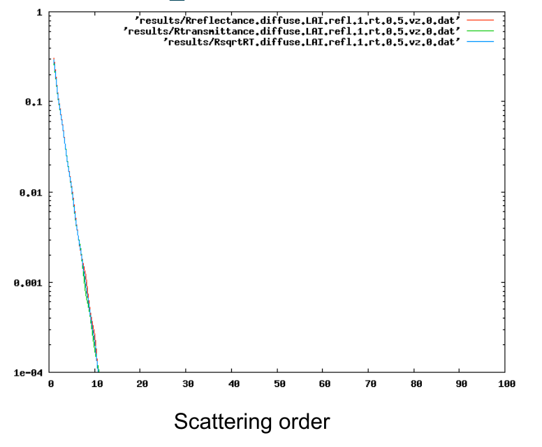
LAI = 1
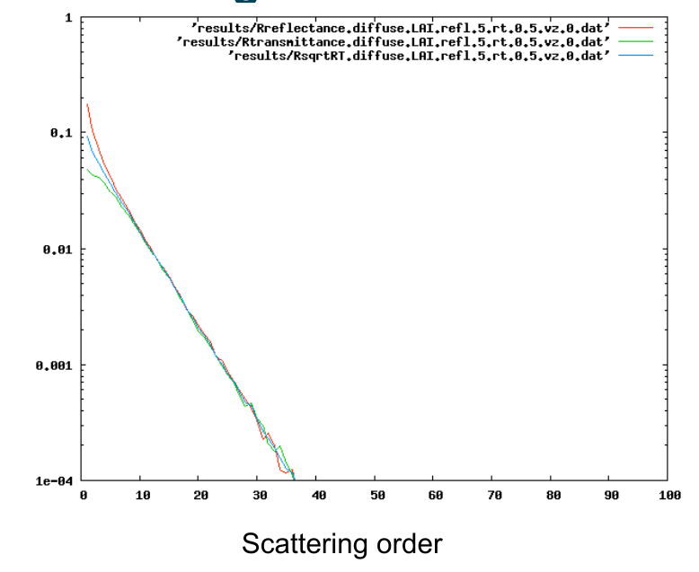
LAI = 5
LAI = 8
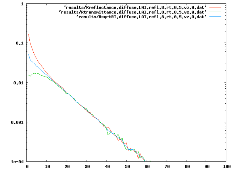
Recollision probability
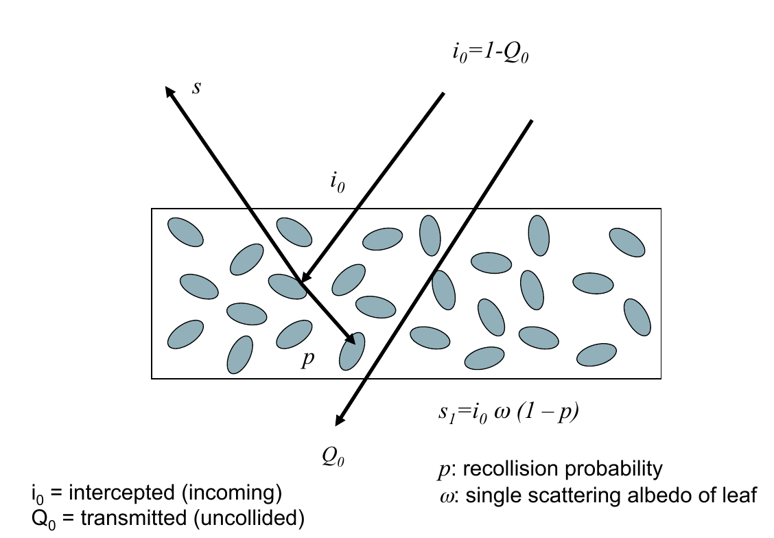
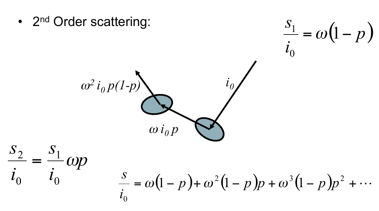
- $p$ is en eigenvalue of the RT equation $\Rightarrow$ only depends on structure
- We can use this form to describe reflectance if black soil (or dense canopy)
- From Smolander & Sternberg (2005),
$$
p = 0.88 \left[ 1 - \exp(- 0.7 LAI^{0.75}) \right]
$$
- Assuming spherical leaf angle distribution
The hotspot effect
- The term $$ \exp\left[-L\frac{G(\vec{\Omega}_s)\mu_o + G(\vec{\Omega}_o)\mu_s}{\mu_s\cdot\mu_o}\right] $$ is usually called the joint gap probability, and is the probability of a photon traversing the canopy downwards and then upwards without a collision.
- We have assumed these two probabilities are independent, which holds in general...
- but what happens if we consider the retroreflection (=backscatter) direction?
- Then, the downward and upward probabilities need to be identical!
- We need a correction factor for the hotspot direction!
- The increased gap probability results in an enhancement of the reflectance factor (the hotspot)
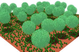
Discontinous canopies
- We have looked at a turbid medium
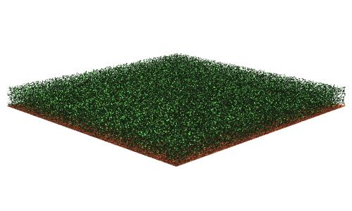
- This might be acceptable for a grass canopy such as cereals
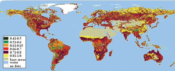
- But clearly not right for a savanna!
- Clumping of the canopoy can be encoded as a modulation on LAI, $C$
So the gap fraction becomes $$ \exp\left(-L\cdot C\frac{G(\Omega)}{\mu}\right) $$
We can think of the LAI of a clumped canopy as being effective if $C\neq1$
- Canopy types:
- Random distribution: For each layer of leaves, there is 37% overlapping. $C=1$.
- Clumped distribution: For each layer ofleaves, there is more than 37% overlapping. $C < 1$
- regular distribution: For each layer of leaves,there is less than 37% overlapping. $C > 1$
Clumping has an effect on the radiation regime inside the canopy
$\Rightarrow$ effect on GPP
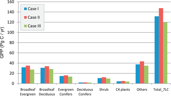
- In the plot
- Case I: LAI and clumping considered
- Case II: clumping considered
- Case III: effective LAI
- Case II vs Case I: ignoring $C$ results in an overestimation of sunlit leaves $\Rightarrow$ increase in GPP
- Case III vs Case I: underestimation of shaded leaf LAI $\Rightarrow$ decrease in GPP
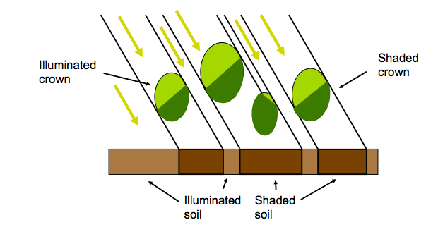
Extending a turbid medium to deal with discontinuous canopies
- Need to deal with the mutual shadowing of e.g. tree crowns, soil, etc. $\Rightarrow$ Geometrical optics (GO)
- A first stage is to assume that crowns are turbid mediums
- Calculate scattering & attenuation
- Deal with shadowing
Using models to "validate" other models
- Hard to measure many processes (e.g. contribution of multiple scattering)
- $\Rightarrow$ use simpler models as a surrogate reality
- $\Rightarrow$ aim here is to understand e.g. effects of assumptions, etc
- RAdiative transfer Model Intercomparison (RAMI)
Summary
- Turbid medium approximation
- 1st O: attenuation & volume scattering
- leaf angle distribution, geometry, LAI...
- Assumptions to make modelling tractable
- Multiple scattering
- $p$-theory
- Hotspot effect
- Discontinuous canopies
- RAMI-type efforts